An adaptive trial is easier to assess when the final result can be
connected back to the interim decisions that led to it. By default,
survival_adapt() returns a one-row trial summary. Set
return_trace = TRUE to retain the summary together with one
record for each completed interim look.
Reviewing one trial’s interim history
This small Bayesian survival design has two interim looks. The treatment arm is assumed to have a lower cumulative failure probability by 24 months.
The common prop_loss = 0.05 specifies a 5% dropout-time
CDF at 24 months. Dropout is exponential and independent of event time
within each arm; an event before dropout remains observed. Actual
dropout censoring can therefore be below 5%, with additional incomplete
follow-up at interim looks due to staged enrollment.
end_of_study <- 24
hazard_control <- prop_to_haz(c(0.20, 0.35), 12, end_of_study)
hazard_treatment <- prop_to_haz(c(0.12, 0.24), 12, end_of_study)

trial <- survival_adapt(
  hazard_treatment = hazard_treatment,
  hazard_control = hazard_control,
  cutpoints = 12,
  N_total = 80,
  lambda = 8,
  lambda_time = NULL,
  interim_look = c(40, 60),
  end_of_study = end_of_study,
  prior_surv = c(0.1, 0.1),
  block = 2,
  rand_ratio = c(control = 1, treatment = 1),
  prop_loss = 0.05,
  alternative = "less",
  h0 = 0,
  Fn = c(0.05, 0.05),
  Sn = c(0.95, 0.90),
  Qn = c(0.99, 0.99),
  prob_ha = 0.95,
  N_impute = 20,
  N_mcmc = 20,
  method = "bayes-surv",
  empty_interval = "prior",
  return_trace = TRUE
)

trial
#> Goldilocks adaptive trial
#>   prob_threshold margin alternative N_treatment N_control N_enrolled N_max
#> 1           0.95      0        less          40        40         80    80
#>   post_prob_ha   est_final ppp_success stop_futility stop_immediate_success
#> 1         0.85 -0.07467928         0.3             0                      0
#>   stop_expected_success trial_success     stopping_reason decision_time
#> 1                     0         FALSE maximum_sample_size      33.09515
#>   accrual_stop_time analysis_ready_time planned_completion_time
#> 1          9.095155            33.09515                33.09515
#>   followup_person_time peak_active_followup
#> 1              1661.71                   76
#>
#> Interim looks completed: 2
The trial summary reports the official outcome and final analysis, when one is required. The interim history provides an audit trail of the predictive probabilities and decisions.
trial$summary
#>   prob_threshold margin alternative N_treatment N_control N_enrolled N_max
#> 1           0.95      0        less          40        40         80    80
#>   post_prob_ha   est_final ppp_success stop_futility stop_immediate_success
#> 1         0.85 -0.07467928         0.3             0                      0
#>   stop_expected_success trial_success     stopping_reason decision_time
#> 1                     0         FALSE maximum_sample_size      33.09515
#>   accrual_stop_time analysis_ready_time planned_completion_time
#> 1          9.095155            33.09515                33.09515
#>   followup_person_time peak_active_followup
#> 1              1661.71                   76
trial$trace
#>   look planned_N calendar_time active_followup N_enrolled N_treatment N_control
#> 1    1        40      4.238838              38         40          20        20
#> 2    2        60      6.628455              57         60          30        30
#>   events_treatment events_control N_pending N_not_enrolled ppp_stop_now
#> 1                0              2        38             40          0.4
#> 2                1              2        57             20          0.3
#>   ppp_stop_now_mcse ppp_stop_now_lower ppp_stop_now_upper ppp_stop_now_draws
#> 1         0.1095445          0.2170686          0.6064151                 20
#> 2         0.1024695          0.1395537          0.5078184                 20
#>   success_threshold immediate_success_threshold immediate_success_crossed
#> 1              0.95                        0.99                     FALSE
#> 2              0.90                        0.99                     FALSE
#>   expected_success_crossed ppp_success_at_max ppp_success_at_max_mcse
#> 1                    FALSE               0.40               0.1095445
#> 2                    FALSE               0.45               0.1112430
#>   ppp_success_at_max_lower ppp_success_at_max_upper ppp_success_at_max_draws
#> 1                0.2170686                0.6064151                       20
#> 2                0.2586506                0.6530686                       20
#>   futility_threshold futility_crossed inner_mc_uncertain_stop_now
#> 1               0.05            FALSE                           8
#> 2               0.05            FALSE                           6
#>   inner_mc_uncertain_success_at_max decision                 decision_reason
#> 1                                 8 continue continue_thresholds_not_crossed
#> 2                                 9 continue continue_thresholds_not_crossed
#>   empty_interval_fallback_count
#> 1                             2
#> 2                             2
#>                                          empty_interval_fallbacks warning_count
#> 1 prior: treatment=0, interval=2 | prior: treatment=1, interval=2             0
#> 2 prior: treatment=0, interval=2 | prior: treatment=1, interval=2             0
#>   warning_messages
#> 1
#> 2
summarise_trial_trace(trial)
#>   interim_looks_completed last_look last_decision final_N final_post_prob_ha
#> 1                       2         2      continue      80               0.85
#>   ppp_stop_now ppp_success_at_max warning_count trial_success
#> 1          0.3               0.45             0         FALSE
For each completed look, ppp_stop_now is the predictive
probability of success if enrollment stops at that look. It is compared
first with immediate_success_threshold and then with
success_threshold. ppp_success_at_max is the
predictive probability of success if enrollment continues to the maximum
sample size and is compared with futility_threshold. The
decision column records whether the design declared
immediate success, stopped accrual for expected success, stopped for
binding futility, or continued.
The interim history retains Monte Carlo summaries rather than every posterior draw or completed imputation. It is therefore concise enough to include in a simulation review or interim-analysis record.
Visualizing the enrollment plan
Trial and simulation results retain their evaluated enrollment
design, so the enrollment projection can be drawn without repeating
lambda, N_total, or the interim looks:
plot_enrollment(
  trial,
  n_sim = 20,
  seed = 20260727,
  time_unit = "months"
)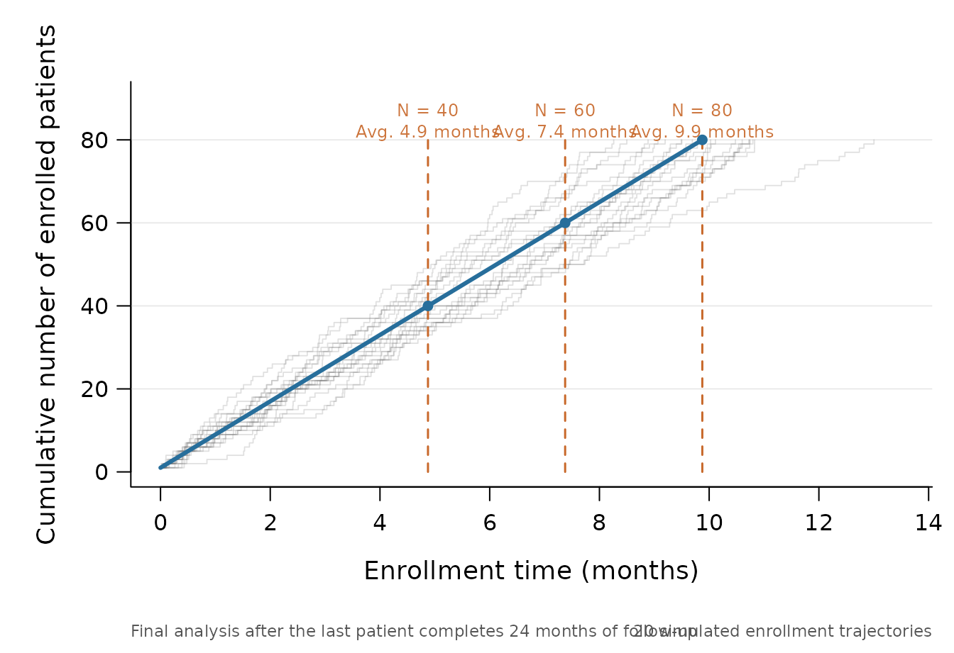
The blue line is expected cumulative enrollment and the grey step
functions are newly simulated enrollment trajectories. Dashed guides
mark the two interim looks and the maximum sample size. Because this
design has a constant enrollment rate, each displayed milestone time is
its mean arrival time, (N - 1) /
\lambda. For piecewise enrollment rates, the plot instead labels
the time at which expected cumulative enrollment reaches the milestone.
Supplying seed makes the displayed enrollment trajectories
reproducible.
Plotting the interim decision path
plot_trial_trace(trial)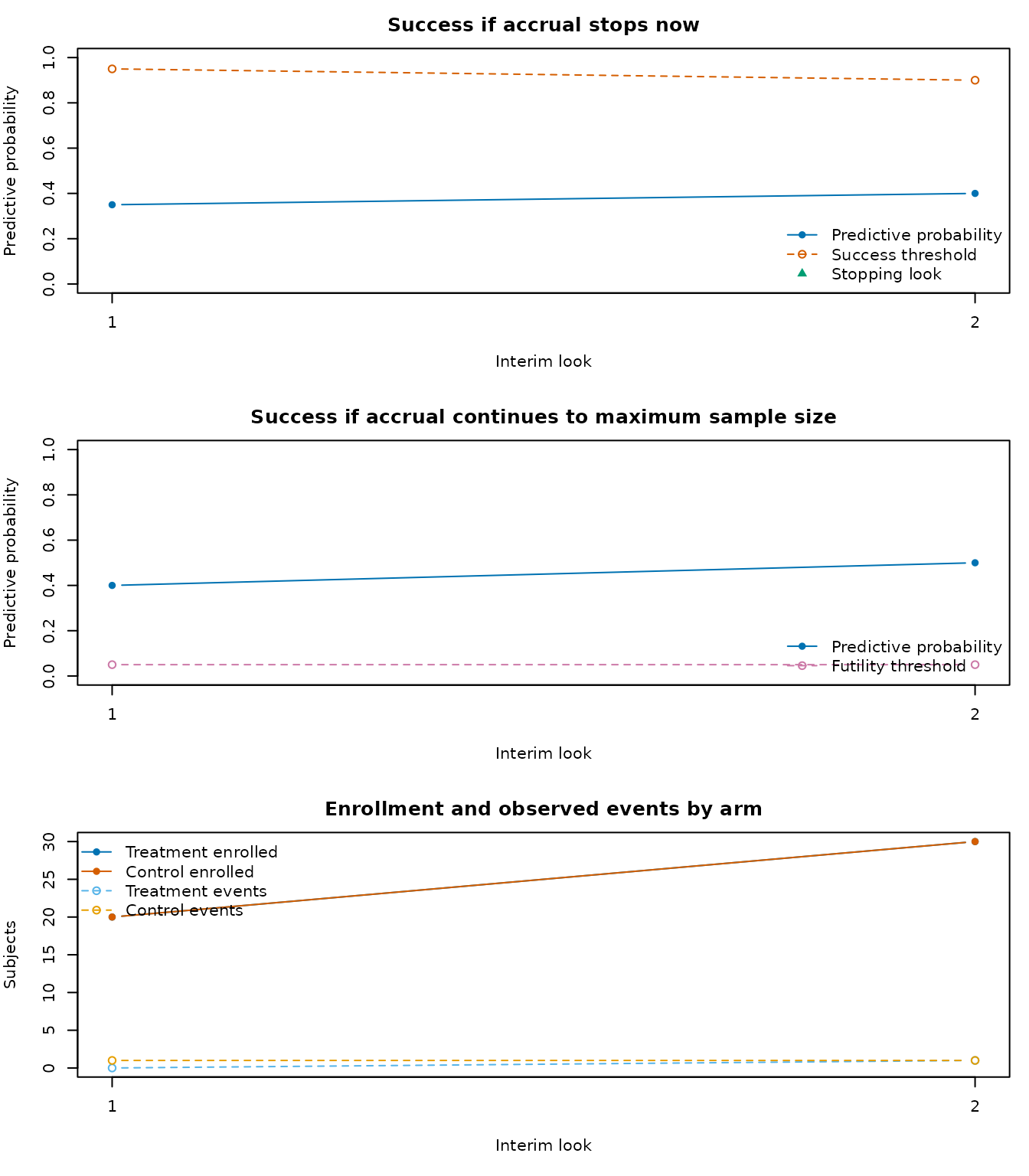
The first two panels show the two predictive probabilities alongside
their decision thresholds. The final panel shows enrollment and observed
events by arm at each look. Warnings raised during a look, such as
empty-interval handling, are recorded in warning_messages
and remain visible as ordinary R warnings.
Summarizing many simulated trials
Interim histories are intended for examining individual trial paths.
By default, sim_trials() retains the trial-level outcomes
needed to estimate operating characteristics. Set
return_trace = TRUE to retain the interim paths as well.
plot_sim_stopping() summarizes where and why enrollment
stopped through marginal, conditional, cumulative, or flowchart views,
while plot_sim_decisions() shows how the two predictive
probabilities map to the decision regions at each look. Supplying the
complete traced result ensures that stopping views include reached looks
at which no trial stopped.
sims <- sim_trials(
  hazard_treatment = hazard_treatment,
  hazard_control = hazard_control,
  cutpoints = 12,
  N_total = 80,
  lambda = 8,
  lambda_time = NULL,
  interim_look = c(40, 60),
  end_of_study = end_of_study,
  prior_surv = c(0.1, 0.1),
  block = 2,
  rand_ratio = c(control = 1, treatment = 1),
  prop_loss = 0.05,
  alternative = "less",
  h0 = 0,
  Fn = c(0.05, 0.05),
  Sn = c(0.95, 0.90),
  Qn = c(0.99, 0.99),
  prob_ha = 0.95,
  N_impute = 20,
  N_mcmc = 20,
  N_trials = 500,
  method = "bayes-surv",
  return_trace = TRUE,
  seed = 5702
)

summarise_sims(sims)
plot_sim_stopping(sims)
plot_sim_stopping(sims, type = "flowchart")
plot_sim_decisions(sims)
The three simulation plotting functions answer different questions.
plot_sim_stopping() describes the terminal sample-size
distribution and can re-express the same stopping paths conditionally,
cumulatively, or as a flow; plot_sim_decisions() explains
how interim predictive probabilities produced those decisions. To
compare operating characteristics across a grid of true treatment
effects, summarize the scenarios together and supply their numeric
effect values to plot_sim_ocs():
scenario_oc <- summarise_sims(list(
  "null" = sims_null,
  "moderate" = sims_moderate,
  "target" = sims
))
effect_by_scenario <- c(null = 0, moderate = -0.05, target = -0.10)
scenario_oc$true_event_probability_difference <- unname(
  effect_by_scenario[scenario_oc$scenario]
)

plot_sim_ocs(
  scenario_oc,
  effect = "true_event_probability_difference",
  xlab = "True treatment-control event-probability difference"
)
For reproducible simulations, prespecify seed in
sim_trials(). Results are then reproducible whether the
trials are evaluated sequentially or in parallel. For a detailed
explanation of the decision algorithm and calibration, see the
“Technical details of the Goldilocks design” vignette.