Normal Mean Estimation with bayesDP

Introduction

The purpose of this vignette is to introduce the bdpnormal function. bdpnormal is used for estimating posterior samples from a Gaussian mean outcome for clinical trials where an informative prior is used. In the parlance of clinical trials, the informative prior is derived from historical data. The weight given to the historical data is determined using what we refer to as a discount function. There are three steps in carrying out estimation:

Estimation of the historical data weight, denoted $\hat{\alpha}$ , via the discount function
Estimation of the posterior distribution of the current data, conditional on the historical data weighted by $\hat{\alpha}$
If a two-arm clinical trial, estimation of the posterior treatment effect, i.e., treatment versus control

Throughout this vignette, we use the terms current, historical, treatment, and control. These terms are used because the model was envisioned in the context of clinical trials where historical data may be present. Because of this terminology, there are 4 potential sources of data:

Current treatment data: treatment data from a current study
Current control data: control (or other treatment) data from a current study
Historical treatment data: treatment data from a previous study
Historical control data: control (or other treatment) data from a previous study

If only treatment data is input, the function considers the analysis a one-arm trial. If treatment data + control data is input, then it is considered a two-arm trial.

Estimation of the historical data weight

In the first estimation step, the historical data weight $\hat{\alpha}$ is estimated. In the case of a two-arm trial, where both treatment and control data are available, an $\hat{\alpha}$ value is estimated separately for each of the treatment and control arms. Of course, historical treatment or historical control data must be present, otherwise $\hat{\alpha}$ is not estimated for the corresponding arm.

When historical data are available, estimation of $\hat{\alpha}$ is carried out as follows. Let $\bar{y}$ , $s$ , and $N$ denote the sample mean, sample standard deviation, and sample size of the current data, respectively. Similarly, let $\bar{y}_0$ , $s_0$ , and $N_0$ denote the sample mean, sample standard deviation, and sample size of the historical data, respectively. Then, the posterior distribution of the mean for current data, under vague (flat) priors is

$\begin{array}{rcl} \tilde{\sigma}^2\mid\bar{y},s,N & \sim & InverseGamma\left(\frac{N-1}{2},\,\frac{N-1}{2}s^2 \right),\\ \\ \tilde{\mu}\mid\bar{y},N,\tilde{\sigma}^2 & \sim & \mathcal{N}ormal\left(\bar{y},\, \frac{1}{N}\tilde{\sigma}^2 \right). \end{array}$

Similarly, the posterior distribution of the mean for historical data, under vague (flat) priors is $\begin{array}{rcl} \sigma^2_0 & \sim & InverseGamma\left(\frac{N_0-1}{2},\,\frac{N_0-1}{2}s_0^2 \right),\\ \\ \mu_0 \mid \bar{y}_0, N_0, \sigma^2_0 & \sim & \mathcal{N}ormal\left(\bar{y}_0,\, \frac{1}{N_0}\sigma^2_0 \right). \end{array}$

We next compute the posterior probability $p = Pr\left(\tilde{\mu} < \mu_0\mid\bar{y},s,N,\bar{y}_0,s_0,N_0\right)$ . Finally, for a discount function, denoted $W$ , $\hat{\alpha}$ is computed as $\hat{\alpha} = \alpha_{max}\cdot W\left(p, \,w\right),\,0\le p\le1,$ where $w$ may be one or more parameters associated with the discount function and $\alpha_{max}$ scales the weight $\hat{\alpha}$ by a user-input maximum value. More details on the discount functions are given in the discount function section below.

There are several model inputs at this first stage. First, the user can select the discount function type via the discount_function input (see below). Next, choosing fix_alpha=TRUE forces a fixed value of $\hat{\alpha}$ (at the alpha_max input), as opposed to estimation via the discount function. In the next modeling stage, a Monte Carlo estimation approach is used, requiring several samples from the posterior distributions. Thus, the user can input a sample size greater than or less than the default value of number_mcmc=10000.

An alternate Monte Carlo-based estimation scheme of $\hat{\alpha}$ has been implemented, controlled by the function input method="mc". Here, instead of treating $\hat{\alpha}$ as a fixed quantity, $\hat{\alpha}$ is treated as random. Because $p$ is recomputed at each Monte Carlo draw using a single pair of posterior samples, the resulting sequence of $\hat{\alpha}$ values can exhibit noticeable Monte Carlo variability. First, $p$ , is computed as

$\begin{array}{rcl} Z & = & \displaystyle{\frac{\left|\tilde{\mu}-\mu_0\right|}{\sqrt{v^2 + v^2_0}}} ,\\ \\ p & = & 2\left(1-\Phi\left(Z\right)\right), \end{array}$ where $\Phi\left(x\right)$ is the $x$ th quantile of a standard normal (i.e., the pnorm R function). Here, $v^2$ and $v^2_0$ are the variances of $\tilde{\mu}$ and $\mu_0$ , respectively. Next, $p$ is used to construct $\hat{\alpha}$ via the discount function. Since the values $Z$ and $p$ are computed at each iteration of the Monte Carlo estimation scheme, $\hat{\alpha}$ is computed at each iteration of the Monte Carlo estimation scheme, resulting in a distribution of $\hat{\alpha}$ values.

Discount function

There are currently three discount functions implemented throughout the bayesDP package. The discount function is specified using the discount_function input with the following choices available:

identity (default): Identity.
weibull: Weibull cumulative distribution function (CDF);
scaledweibull: Scaled Weibull CDF;

First, the identity discount function (default) sets the discount weight $\hat{\alpha}=p$ .

Second, the Weibull CDF has two user-specified parameters associated with it, the shape and scale. The default shape is 3 and the default scale is 0.135, each of which are controlled by the function inputs weibull_shape and weibull_scale, respectively. The form of the Weibull CDF is $W(x) = 1 - \exp\left\{- (x/w_{scale})^{w_{shape}}\right\}.$

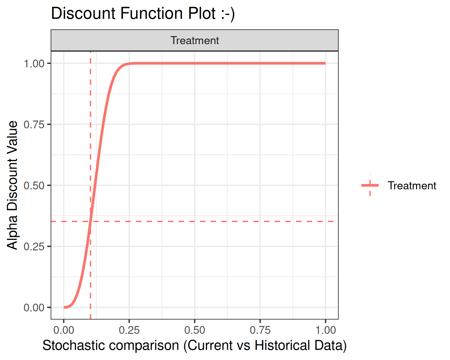
The third discount function option is the Scaled Weibull CDF. The Scaled Weibull CDF is the Weibull CDF divided by the value of the Weibull CDF evaluated at 1, i.e., $W^{\ast}(x) = W(x)/W(1).$ Similar to the Weibull CDF, the Scaled Weibull CDF has two user-specified parameters associated with it, the shape and scale, again controlled by the function inputs weibull_shape and weibull_scale, respectively.

Using the default shape and scale inputs, each of the discount functions are shown below.

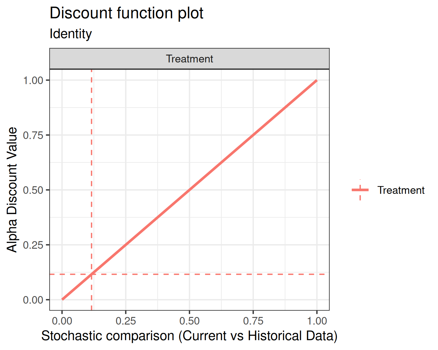
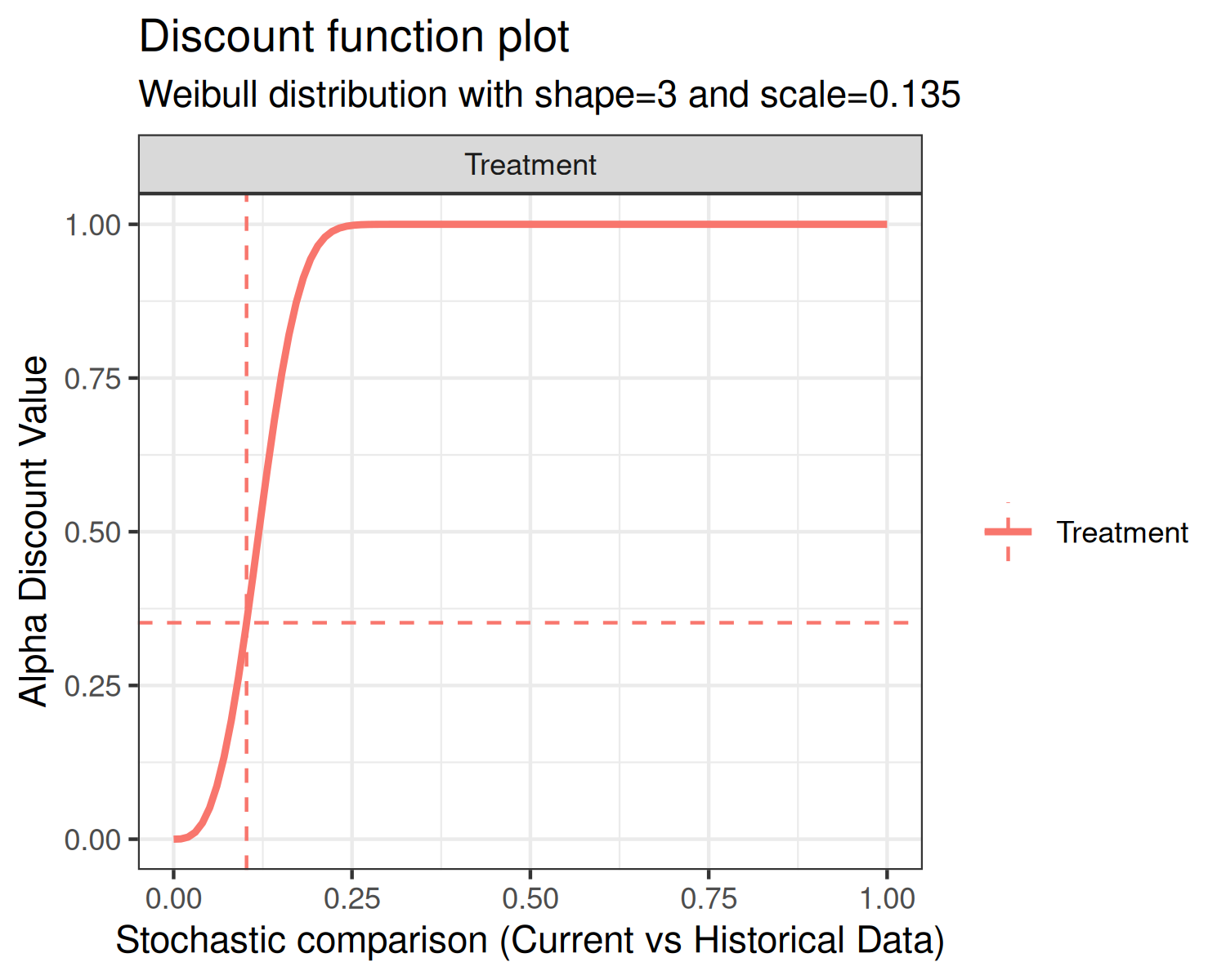
In each of the above plots, the x-axis is the stochastic comparison between current and historical data, which we’ve denoted $p$ . The y-axis is the discount value $\hat{\alpha}$ that corresponds to a given value of $p$ .

An advanced input for the plot function is print. The default value is print = TRUE, which simply returns the graphics. Alternately, users can specify print = FALSE, which returns a ggplot2 object. Below is an example using the discount function plot:

p1 <- plot(fit02, type="discount", print=FALSE)
p1 + ggtitle("Discount Function Plot :-)")

Estimation of the posterior distribution of the current data, conditional on the historical data

With $\hat{\alpha}$ in hand, we can now estimate the posterior distribution of the mean of the current data. Using the notation of the previous section, the posterior distribution is $\mu \sim \mathcal{N}ormal\left( \frac{\sigma^2_0N\bar{y} + \tilde{\sigma}^2N_0\bar{y}_0\hat{\alpha}}{N\sigma^2_0 + \tilde{\sigma}^2N_0\hat{\alpha}},\,\frac{\tilde{\sigma}^2\sigma^2_0}{N\sigma^2_0 + \tilde{\sigma}^2N_0\hat{\alpha}} \right).$ At this model stage, we have in hand number_mcmc simulations from the augmented mean distribution. If there are no control data, i.e., a one-arm trial, then the modeling stops and we generate summaries of the posterior distribution of $\mu$ . Otherwise, if there are control data, we proceed to a third step and compute a comparison between treatment and control data.

Estimation of the posterior treatment effect: treatment versus control

This step of the model is carried out on-the-fly using the summary or print methods. Let $\mu_T$ and $\mu_C$ denote posterior mean estimates of the treatment and control arms, respectively. Currently, the implemented comparison between treatment and control is the difference, i.e., summary statistics related to the posterior difference: $\mu_T - \mu_C$ . In a future release, we may consider implementing additional comparison types.

Inputting Data

The data inputs for bdpnormal are mu_t, sigma_t, N_t, mu0_t, sigma0_t, N0_t, mu_c, sigma_c, N_c, mu0_c, sigma0_c, and N0_c. The data must be input as (mu, sigma, N) triplets. For example, mu_t, the sample mean of the current treatment group, must be accompanied by sigma_t and N_t, the sample standard deviation and sample size, respectively. Historical data inputs are not necessary, but using this function would not be necessary either.

At the minimum, mu_t, sigma_t, and N_t must be input. In the case that only mu_t, sigma_t, and N_t are input, the analysis is analogous to a one-sample t-test. Each of the following input combinations are allowed:

(mu_t, sigma_t, N_t) - one-arm trial
(mu_t, sigma_t, N_t) + (mu0_t, sigma0_t, N0_t) - one-arm trial
(mu_t, sigma_t, N_t) + (mu_c, sigma_c, N_c) - two-arm trial
(mu_t, sigma_t, N_t) + (mu0_c, sigma0_c, N0_c) - two-arm trial
(mu_t, sigma_t, N_t) + (mu0_t, sigma0_t, N0_t) + (mu_c, sigma_c, N_c) - two-arm trial
(mu_t, sigma_t, N_t) + (mu0_t, sigma0_t, N0_t) + (mu0_c, sigma0_c, N0_c) - two-arm trial
(mu_t, sigma_t, N_t) + (mu0_t, sigma0_t, N0_t) + (mu_c, sigma_c, N_c) + (mu0_c, sigma0_c, N0_c) - two-arm trial

Examples

One-arm trial

Suppose we have historical data with a mean of mu0_t=50, standard deviation of sigma0_t=10, and sample size of N0_t=50 patients. Also suppose that we have current data with a mean of mu_t=45, standard deviation of sigma_t=10, and sample size of N_t=50. To illustrate the approach, let’s first give full weight to the historical data. This is accomplished by setting alpha_max=1 and fix_alpha=TRUE as follows:

set.seed(42)
fit1 <- bdpnormal(mu_t      = 45,
                  sigma_t   = 10,
                  N_t       = 50, 
                  mu0_t     = 50,
                  sigma0_t  = 10,
                  N0_t      = 50,
                  alpha_max = 1,
                  fix_alpha = TRUE,
                  method    = "fixed")
summary(fit1)

## 
##     One-armed bdp normal
## 
## data:
##   Current treatment: mu_t = 45, sigma_t = 10, N_t = 50
##   Historical treatment: mu0_t = 50, sigma0_t = 10, N0_t = 50
## Stochastic comparison (p_hat) - treatment (current vs. historical data): 0.0134
## Discount function value (alpha) - treatment: 1
## 95 percent CI: 
##  45.4329  49.6303
## posterior sample estimate:
## mean of treatment group
##  47.5208

Based on the summary output of fit1, we can see that the value of alpha was held fixed at 1. Note that the print and summary methods result in the same output. The resulting treatment group mean is approximately 47.5, which is the average of 45 and 50, as expected.

Now, let’s relax the constraint on fixing alpha at 1 and let the function estimate alpha. We’ll also take this opportunity to describe the output of the plot method.

set.seed(42)
fit1a <- bdpnormal(mu_t      = 45, sigma_t  = 10, N_t  = 50, 
                   mu0_t     = 50, sigma0_t = 10, N0_t = 50,
                   fix_alpha = FALSE,
                   method    = "fixed")
summary(fit1a)

## 
##     One-armed bdp normal
## 
## data:
##   Current treatment: mu_t = 45, sigma_t = 10, N_t = 50
##   Historical treatment: mu0_t = 50, sigma0_t = 10, N0_t = 50
## Stochastic comparison (p_hat) - treatment (current vs. historical data): 0.0134
## Discount function value (alpha) - treatment: 0.0134
## 95 percent CI: 
##  42.2972  47.9262
## posterior sample estimate:
## mean of treatment group
##  45.0795

When alpha is not constrained to one, it is estimated based on a comparison between the current and historical data. We see that the stochastic comparison, p_hat, between current historical and control is 0.0134. Here, p_hat is the posterior probability of the comparison between the current and historical data. With the present example, the low value of p_hat implies that the current and historical sample means are different. The result is that the weight given to the historical data is shrunk towards zero. Thus, the estimate of alpha from the discount function is 0.0134 and the augmented posterior estimate of the mean is approximately the mean of the current data.

Many of the the values presented in the summary method are accessible from the fit object. For instance, alpha is found in fit1a$posterior_treatment$alpha_discount and p_hat is located at fit1a$posterior_treatment$p_hat. The augmented mean and CI are computed at run-time. The results can be replicated as:

mean_augmented <- round(median(fit1a$posterior_treatment$posterior_mu),4)
mean_augmented

## [1] 45.0795

CI95_augmented <- round(quantile(fit1a$posterior_treatment$posterior_mu, prob=c(0.025, 0.975)),4)
CI95_augmented

##    2.5%   97.5% 
## 42.2972 47.9262

Finally, we’ll explore the plot method.

plot(fit1a, type="posteriors")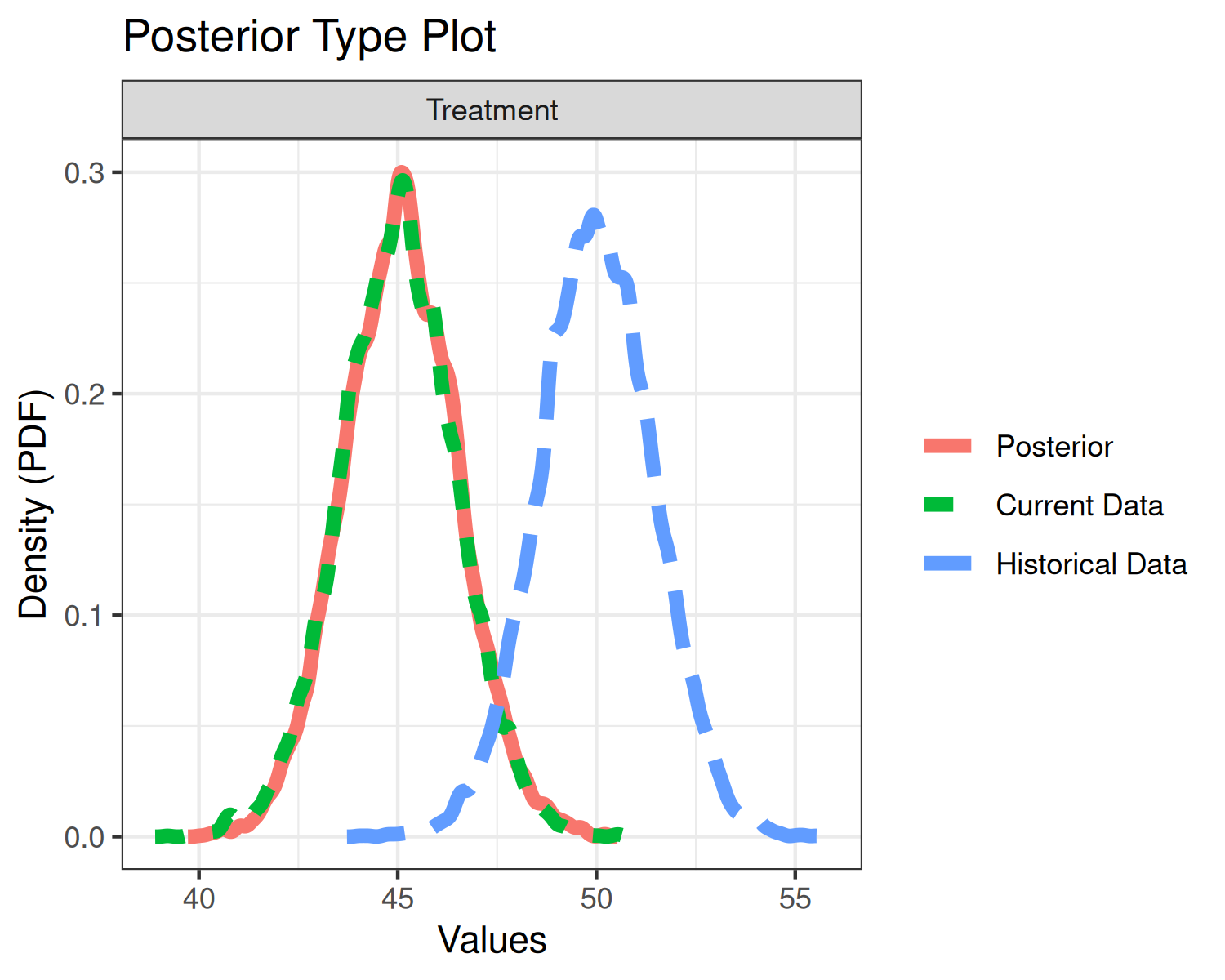

plot(fit1a, type="density")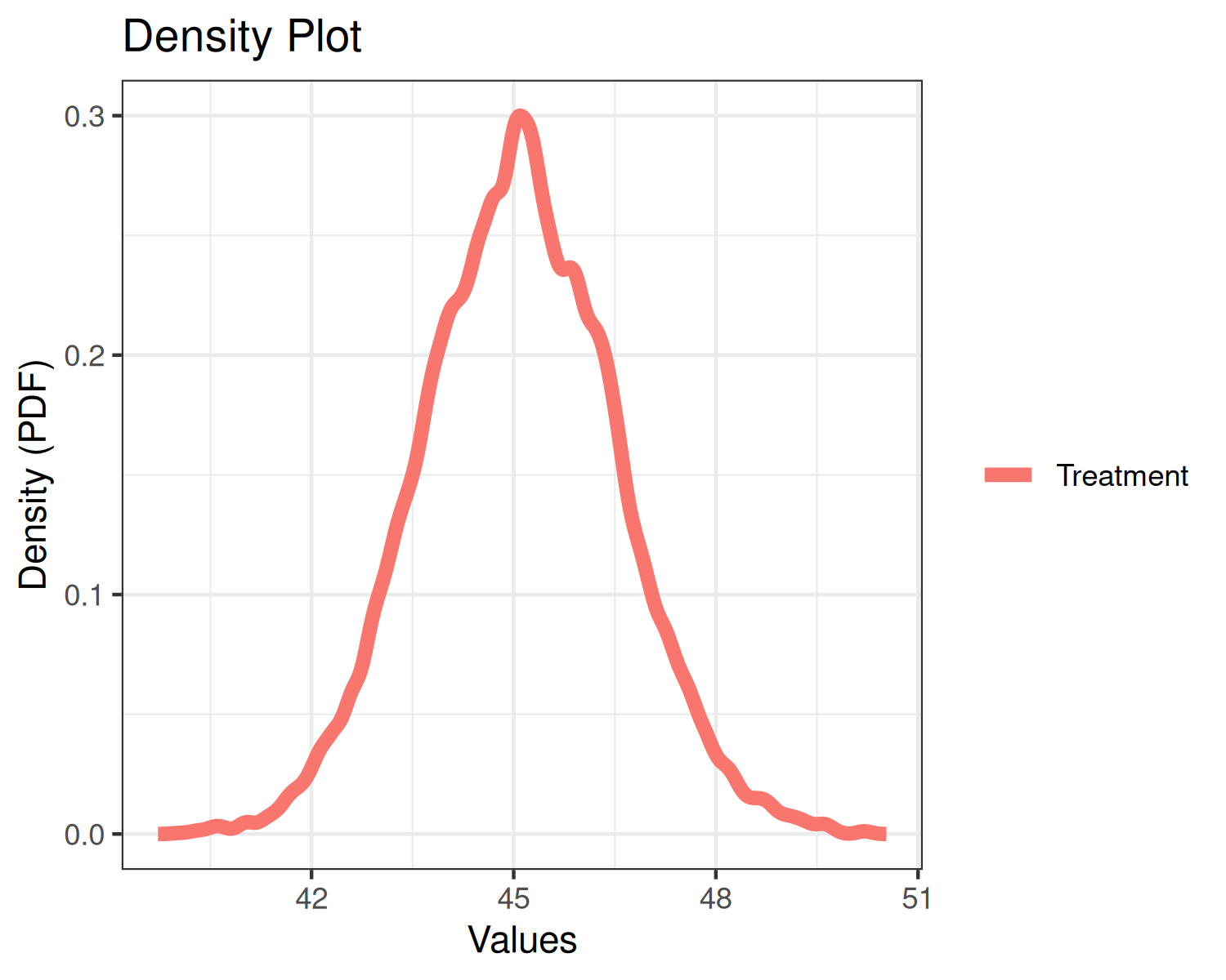

plot(fit1a, type="discount")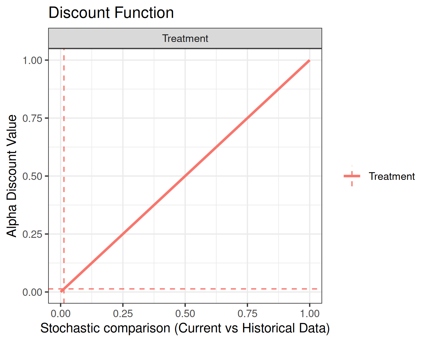

The top plot displays three density curves. The blue curve is the density of the historical mean, the green curve is the density of the current mean, and the red curve is the density of the current mean augmented by historical data. Since little weight was given to the historical data, the current and posterior means essentially overlap.

The middle plot simply re-displays the posterior mean.

The bottom plot displays the discount function (solid curve) as well as alpha (horizontal dashed line) and p_hat (vertical dashed line). In the present example, the discount function is the identity.

Two-arm trial

On to two-arm trials. In this package, we define a two-arm trial as an analysis where a current and/or historical control arm is present. Suppose we have the same treatment data as in the one-arm example, but now we introduce control data: mu_c = 40, sigma_c = 10, N_c = 50, mu0_c = 40, sigma0_c = 10, and N0_c = 50.

Before proceeding, it is worth pointing out that the discount function is applied separately to the treatment and control data. Now, let’s carry out the two-arm analysis using default inputs:

set.seed(42)
fit2 <- bdpnormal(mu_t      = 45, sigma_t  = 10, N_t  = 50, 
                  mu0_t     = 50, sigma0_t = 10, N0_t = 50,
                  mu_c      = 40, sigma_c  = 10, N_c  = 50, 
                  mu0_c     = 40, sigma0_c = 10, N0_c = 50,
                  fix_alpha = FALSE,
                  method    = "fixed")
summary(fit2)

## 
##     Two-armed bdp normal
## 
## data:
##   Current treatment: mu_t = 45, sigma_t = 10, N_t = 50
##   Current control: mu_c = 40, sigma_c = 10, N_c = 50
##   Historical treatment: mu0_t = 50, sigma0_t = 10, N0_t = 50
##   Historical control: mu0_c = 40, sigma0_c = 10, N0_c = 50
## Stochastic comparison (p_hat) - treatment (current vs. historical data): 0.0134
## Stochastic comparison (p_hat) - control (current vs. historical data): 0.9922
## Discount function value (alpha) - treatment: 0.0134
## Discount function value (alpha) - control: 0.9922
## alternative hypothesis: two.sided
## 95 percent CI: 
##  1.7412  8.5362
## posterior sample estimates:
## treatment group  control group
##           45.08          40.01

The summary method of a two-arm analysis is slightly different than a one-arm analysis. First, we see p_hat and alpha reported for the control data. In the present analysis, the current and historical control data have sample means that are very close, thus the historical control data is given nearly full weight. Again, little weight is given to the historical treatment data.

The CI is computed at run time and is the interval estimate of the difference between the posterior means of the treatment and control groups. With a 95% CI of (1.7412, 8.5362), we would conclude that the treatment and control arms are not significantly different since zero is outside of the CI.

The plot method of a two-arm analysis is slightly different than a one-arm analysis as well:

plot(fit2, type="posteriors")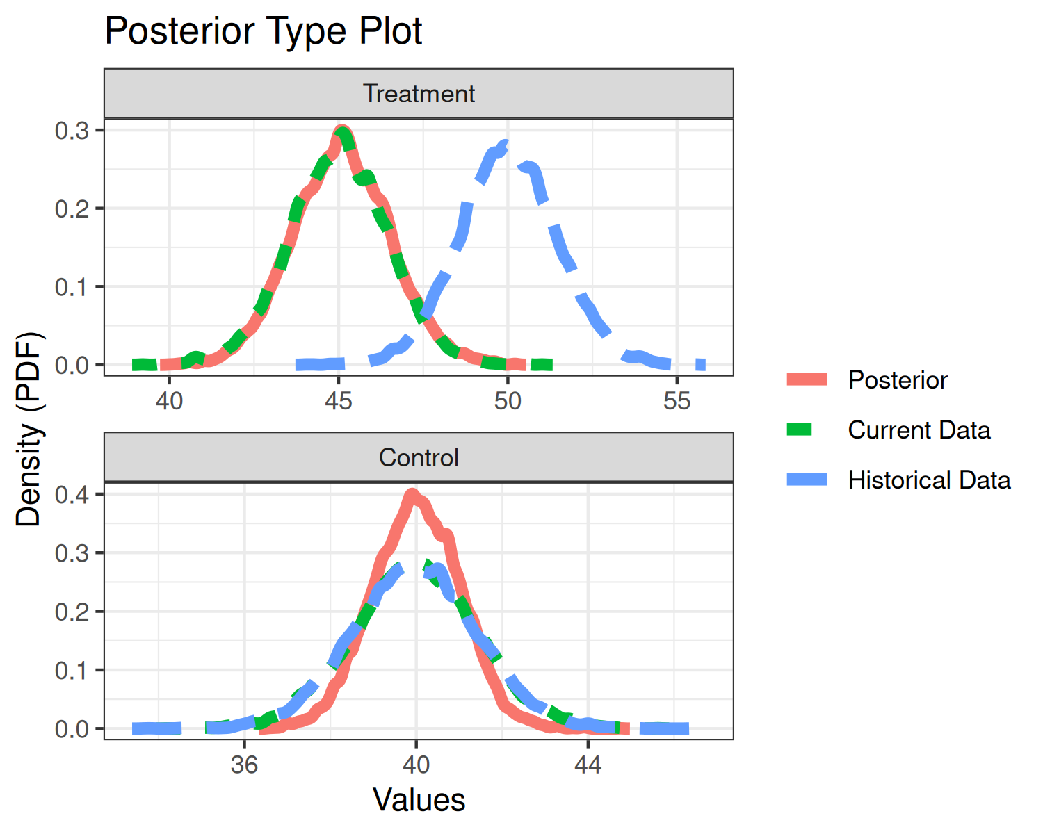

plot(fit2, type="density")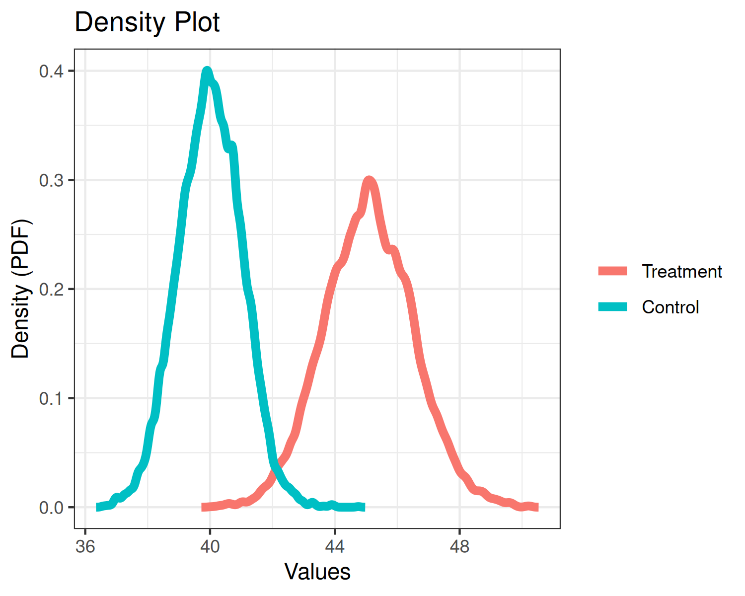

plot(fit2, type="discount")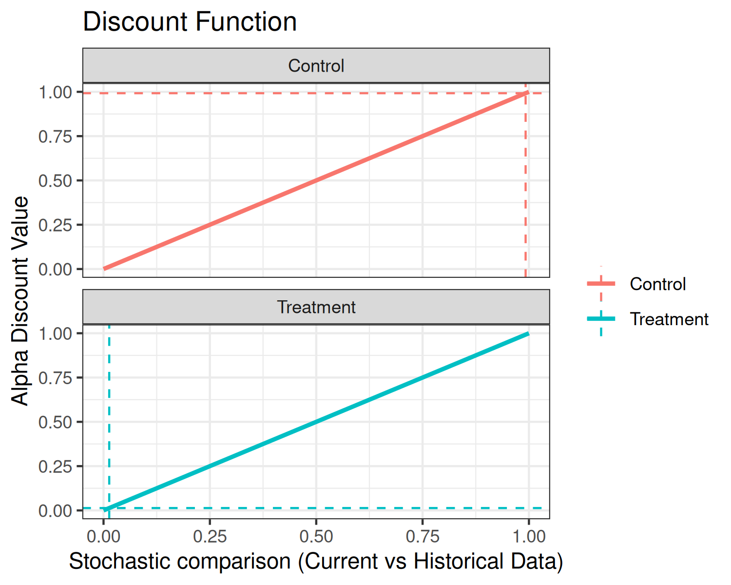

Each of the three plots are analogous to the one-arm analysis, but each plot now presents additional data related to the control arm.

Donnie Musgrove

2026-06-25