Linear Regression Estimation with bayesDP

Introduction

The purpose of this vignette is to introduce the bdplm function. bdplm is used for estimating posterior samples in the context of linear regression for clinical trials where an informative prior is used. In the parlance of clinical trials, the informative prior is derived from historical data. The weight given to the historical data is determined using what we refer to as a discount function. There are three steps in carrying out estimation:

Estimation of the historical data weight, denoted $\hat{\alpha}$ , via the discount function
Estimation of the posterior distribution of the current data, conditional on the historical data weighted by $\hat{\alpha}$
Estimation of the posterior treatment effect, i.e., treatment versus control

Throughout this vignette, we use the terms current, historical, treatment, and control. These terms are used because the model was envisioned in the context of clinical trials where historical data may be present. Because of this terminology, there are 4 potential sources of data:

Current treatment data: treatment data from a current study
Current control data: control (or other treatment) data from a current study
Historical treatment data: treatment data from a previous study
Historical control data: control (or other treatment) data from a previous study

If only treatment data is input, the function considers the analysis a one-arm trial. If treatment data + control data is input, then it is considered a two-arm trial.

Note that the bdplm function currently only has support for a two-arm clinical trial where current and historical treatment and current and historical control data are all present.

Linear Regresion Model Background

Before we get into our estimation scheme, we will briefly describe our implementation of the linear regression model. The linear regression model implementation, via bdplm, serves as an advanced companion to the bdpnormal model. With the bdpnormal model, we are interested in comparing mean outcomes via the probability that the mean values from treatment and control arms are not equivalent. When covariate adjustments are needed, bdpnormal is no longer a viable solution. Thus, bdplm allows analysts to adjust the treatment and control arm comparison for covariate effects.

The analysis model of interest has the form $y_i = \beta_0 + \beta_1I(treatment_i) + x_{2i}\beta_2 + \cdots+x_{mi}\beta_m + \varepsilon_i, \varepsilon_i \sim \mathcal{N}ormal\left(0,\,\sigma^2\right),\,\,\,i=1,\dots,n,$ where $I(treatment_i)$ indicates whether observation $i$ is in the treatment arm, $\beta_0$ is the intercept, $\beta_1$ is the treatment effect, $x_{ji}$ is the $j$ th covariate with corresponding $\beta_j$ covariate effect, $j=2,\dots,m$ , and $\sigma^2$ is the unknown error variance.

Let $\boldsymbol{x}_i^T\boldsymbol{\beta}_{-(0,1)} = x_{2i}\beta_2 + \cdots+x_{mi}\beta_m$ . Then, in order to place prior values on the treatment effect, we reparameterize the linear regression model as $y_i = \beta_0^{\ast}I(control_i) + \beta_1^{\ast}I(treatment_i) + \boldsymbol{x}_i^T\beta_{-(0,1)} + \varepsilon_i, \varepsilon_i \sim \mathcal{N}ormal\left(0,\,\sigma^2\right),\,\,\,i=1,\dots,n,$ where now $I(control_i)$ indicates whether observation $i$ is in the control arm, i.e., $I(control_i) = 1 - I(treatment_i)$ . It is then straightforward to show that $\beta_0 = \beta^{\ast}_0$ and $\beta_1 = \beta_1^{\ast} - \beta^{\ast}_0$ .

In this reparameterization, $\beta_0^{\ast}$ and $\beta_1^{\ast}$ are the control and treatment arm means evaluated at covariate $= 0$ . When the covariates are not centered, these arm-mean parameters become strongly correlated and their (historical) standard errors are extrapolation errors at covariate $= 0$ . Because the historical information is incorporated through an independent (diagonal) prior on each arm mean, this correlation and the inflated standard errors distort the borrowing of historical data. To avoid this, bdplm automatically mean-centers each covariate on its pooled (current plus historical) mean before fitting, so that $\beta_0^{\ast}$ and $\beta_1^{\ast}$ are the arm means at the average covariate value. The intercept is then back-transformed onto the original covariate scale: with pooled covariate means $\bar{x}_j$ and estimated covariate effects $\beta_j$ , the reported intercept is $\beta_0 = \beta_0^{\ast} - \sum_j \beta_j\bar{x}_j$ , so $\beta_0$ is still the control mean at covariate $= 0$ on the original scale. The treatment effect $\beta_1$ and the covariate effects are unchanged by centering, and the estimates are invariant to a location shift of any covariate. Users therefore do not need to center covariates themselves.

Estimation of the historical data weight

In the first estimation step, the historical data weight $\hat{\alpha}$ is estimated. In the case of a two-arm trial, where both treatment and control data are available, an $\hat{\alpha}$ value is estimated separately for each of the treatment and control arms. Of course, historical treatment or historical control data must be present, otherwise $\hat{\alpha}$ is not estimated for the corresponding arm.

When historical data are available, estimation of $\hat{\alpha}$ is carried out as follows. Let $\boldsymbol{y}$ and $\boldsymbol{y}_0$ denote the current and historical data, respectively. The following linear regression model is then fit to the data: $y_i = \tilde{\beta}_0 + \tilde{\beta}_1I(historical_i) + x_{2i}\tilde{\beta}_2 + \cdots+x_{mi}\tilde{\beta}_m + \varepsilon_i, \varepsilon_i \sim \mathcal{N}ormal\left(0,\,\sigma^2\right),\,\,\,i=1,\dots,n,$ where $I(historical_i)$ indicates whether observation $i$ is historical. With vague priors on each parameter, we estimate the posterior probability that $\tilde{\beta}_1 > 0$ by first computing $p_1 = Pr\left(\tilde{\beta_1} > 0 \mid \boldsymbol{y}, \boldsymbol{y}_0\right)$ . Then, we calculate the posterior probability $p$ as

$p=\begin{cases} 2p_{1}, & p_{1}\le0.5\\ 2\left(1-p_{1}\right), & p_{1}>0.5. \end{cases}$

Finally, for a discount function, denoted $W$ , $\hat{\alpha}$ is computed as $\hat{\alpha} = \alpha_{max}\cdot W\left(p, \,w\right),\,0\le p\le1,$ where $w$ may be one or more parameters associated with the discount function and $\alpha_{max}$ scales the weight $\hat{\alpha}$ by a user-input maximum value. More details on the discount functions are given in the discount function section below.

There are several model inputs at this first stage. First, the user can select fix_alpha=TRUE and force a fixed value of $\hat{\alpha}$ (at the alpha_max input), as opposed to estimation via the discount function.

An alternate Monte Carlo-based estimation scheme of $\hat{\alpha}$ has been implemented, controlled by the function input method="mc". Here, instead of treating $\hat{\alpha}$ as a fixed quantity, $\hat{\alpha}$ is treated as random. First, $p$ , is computed as

$\begin{array}{rcl} Z & = & \displaystyle{\frac{\left|\beta_1\right|}{\sigma_{\beta}}},\\ \\ p & = & 2\left(1-\Phi\left(Z\right)\right), \end{array}$ where $\sigma_{\beta}$ is an estimate of the standard deviation of $\beta_1$ and $\Phi\left(x\right)$ is the $x$ th quantile of a standard normal (i.e., the pnorm R function). Next, $p$ is used to construct $\hat{\alpha}$ via the discount function. Since the values $Z$ and $p$ are computed at each iteration of the Monte Carlo estimation scheme, $\hat{\alpha}$ is computed at each iteration of the Monte Carlo estimation scheme, resulting in a distribution of $\hat{\alpha}$ values.

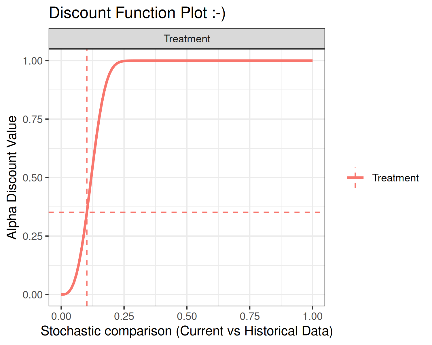
Discount function

There are currently three discount functions implemented throughout the bayesDP package. The discount function is specified using the discount_function input with the following choices available:

identity (default): Identity.
weibull: Weibull cumulative distribution function (CDF);
scaledweibull: Scaled Weibull CDF;

First, the identity discount function (default) sets the discount weight $\hat{\alpha}=p$ .

Second, the Weibull CDF has two user-specified parameters associated with it, the shape and scale. The default shape is 3 and the default scale is 0.135, each of which are controlled by the function inputs weibull_shape and weibull_scale, respectively. The form of the Weibull CDF is $W(x) = 1 - \exp\left\{- (x/w_{scale})^{w_{shape}}\right\}.$

The third discount function option is the Scaled Weibull CDF. The Scaled Weibull CDF is the Weibull CDF divided by the value of the Weibull CDF evaluated at 1, i.e., $W^{\ast}(x) = W(x)/W(1).$ Similar to the Weibull CDF, the Scaled Weibull CDF has two user-specified parameters associated with it, the shape and scale, again controlled by the function inputs weibull_shape and weibull_scale, respectively.

Using the default shape and scale inputs, each of the discount functions are shown below.

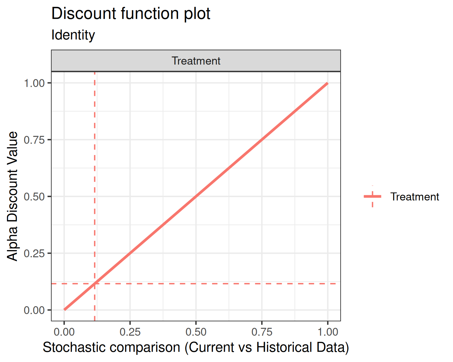
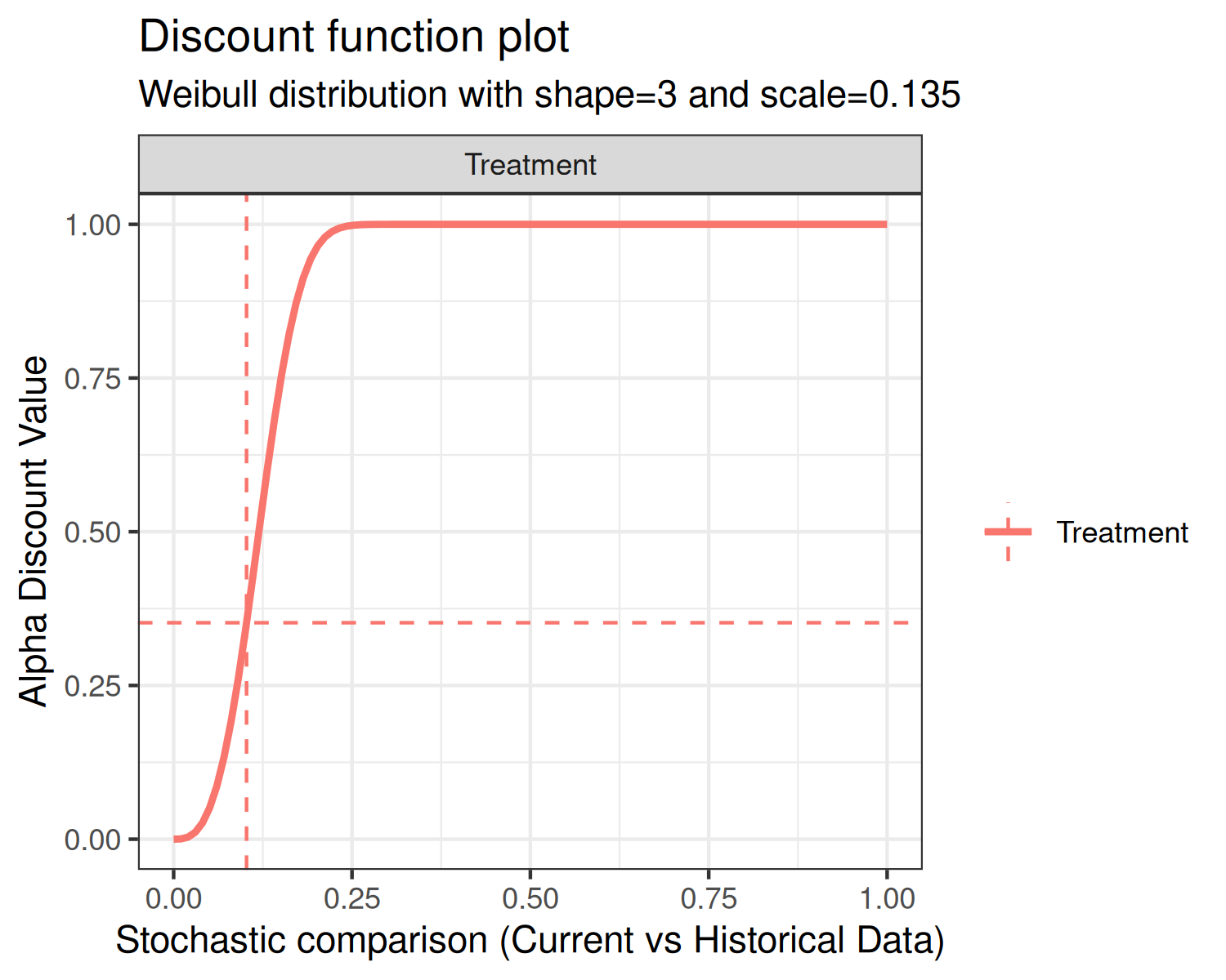
In each of the above plots, the x-axis is the stochastic comparison between current and historical data, which we’ve denoted $p$ . The y-axis is the discount value $\hat{\alpha}$ that corresponds to a given value of $p$ .

An advanced input for the plot function is print. The default value is print = TRUE, which simply returns the graphics. Alternately, users can specify print = FALSE, which returns a ggplot2 object. Below is an example using the discount function plot:

p1 <- plot(fit02, type="discount", print=FALSE)
p1 + ggtitle("Discount Function Plot :-)")

Estimation of the posterior distribution of the current data, conditional on the historical data

This section details the modeling scheme used to estimate the parameters of the linear regression model. In vector notation the model can be written $$ \begin{array}{rcl} \mathbf{y} & \sim & \mathcal{N}\left(\mathbf{X}\boldsymbol{\beta},\thinspace\boldsymbol{\Sigma}_{y}\right),\\ \\ \boldsymbol{\beta} & \sim & \mathcal{N}\left(\boldsymbol{\mu}_{\beta},\thinspace\boldsymbol{\Sigma}_{\beta}\right), \end{array} $$ where $\boldsymbol{\mu}_{\beta}=\left(\mu_0,\,\mu_1,\,\mu_2,\dots,\,\mu_m\right)^T$ and $\boldsymbol{\Sigma}_{\beta}=\mbox{diag}\left(\tau^2_0/\alpha_{00},\,\tau^2_1/\alpha_{01},\,\tau^2_2,\dots,\tau^2_m\right)$ are known and $\boldsymbol{\Sigma}_y=\sigma^2\mathbf{I}_n$ . Here, $\mu_0$ and $\mu_1$ are the prior means of the control and treatment effects, respectively, while $\mu_2,\dots,\,\mu_m$ are the prior means of the covariate effects. Likewise, $\tau^2_0/\alpha_{00}$ and $\tau^2_1/\alpha_{01}$ are the prior variances of the control and treatment effects (weighted by the discount function result $\alpha$ ), respectively, while $\tau^2_2,\dots,\tau^2_m$ are the prior variances of the remaining covariate effects.

Using what we refer to as the Gelman parameterization (see Gelman’s Bayesian Data Analysis, 3rd edition, chapter 14, for more information), the model can be reparameterized to improve computational efficiency. First, write $$ \mathbf{y}_{\ast}=\left(\begin{array}{c} \mathbf{y}\\ \boldsymbol{\mu}_{\beta} \end{array}\right),\thinspace\mathbf{X}_{\ast}=\left(\begin{array}{c} \mathbf{X}\\ \mathbf{I}_m \end{array}\right),\thinspace\boldsymbol{\Sigma}_{\ast}=\left(\begin{array}{cc} \boldsymbol{\Sigma}_y & 0\\ 0 & \boldsymbol{\Sigma}_{\beta} \end{array}\right). $$ Then, the Gelman parameterization has the form $\mathbf{y}_{\ast}=\mathbf{X}_{\ast}\boldsymbol{\beta}+\boldsymbol{\varepsilon},\,\,\,\boldsymbol{\varepsilon}\sim\mathcal{N}\left(\mathbf{0},\,\boldsymbol{\Sigma}_{\ast}\right).$ The estimate of $\boldsymbol{\beta}$ is computed as $\hat{\boldsymbol{\beta}}=\mathbf{V}_{\beta}\mathbf{X}_{\ast}^T\boldsymbol{\Sigma}_{\ast}^{-1}\mathbf{y}_{\ast},$ where $\mathbf{V}_{\beta}=\left(\mathbf{X}_{\ast}^T\boldsymbol{\Sigma}_{\ast}^{-1}\mathbf{X}_{\ast}\right)^{-1}.$ This estimate of $\hat{\boldsymbol{\beta}}$ is the posterior mean and relies on an unknown parameter, $\sigma^2$ . The marginal posterior distribution of $\sigma^2$ is found as $\begin{array}{rcl} \pi\left(\sigma^2\mid\mathbf{y}\right) & \propto & {\displaystyle \left(\frac{1}{\sigma^2}\right)^{n/2+1}\left|\mathbf{V}_{\beta}\right|^{1/2}\exp\left\{ -\frac{1}{2}\left(\mathbf{y}_{\ast}-\mathbf{X}_{\ast}\hat{\boldsymbol{\beta}}\right)^T\boldsymbol{\Sigma}_{\ast}^{-1}\left(\mathbf{y}_{\ast}-\mathbf{X}_{\ast}\hat{\boldsymbol{\beta}}\right)\right\} }. \end{array}$ Notice that both $\mathbf{V}_{\beta}$ and $\Sigma_{\ast}$ contain $\sigma^2$ . Thus, this marginal posterior of $\sigma^2$ does not have a known distribution. We resort to a grid search of $\sigma^2$ where 100s or 1000s of values of $\sigma^2$ are proposed, on a grid, and the proposed values are sampled with probability proportional to the likelihood evaluated at the proposal.

Finally, values of $\sigma^2$ sampled from the posterior distribution are then used to sample values of $\boldsymbol{\beta}$ from $\boldsymbol{\beta} \sim \mathcal{N}\left(\hat{\boldsymbol{\beta}},\, \mathbf{V}_{\beta}\right).$

Inputting Data

The data inputs for bdplm are via dataframes data and data0 that must have matching column names. Each dataframe must have a binary column named treatment that indicates treatment vs. control. If no covariate columns are present, users should use the bdpnormal function. Currently, both data and data0 must be input since only a two-armed clinical trial with historical data has been implemented.

Examples

Two-arm trial

Throughout this package, we define a two-arm trial as an analysis where a current and/or historical control arm is present. Below we simulate a dataframe and view the estimates of the model fit.

set.seed(42)
### Simulate  data
# Sample sizes
n_t  <- 30     # Current treatment sample size
n_c  <- 30     # Current control sample size
n_t0 <- 80     # Historical treatment sample size
n_c0 <- 80     # Historical control sample size

# Treatment group vectors for current and historical data
treatment   <- c(rep(1,n_t), rep(0,n_c))
treatment0  <- c(rep(1,n_t0), rep(0,n_c0))

# Simulate a covariate effect for current and historical data
x  <- rnorm(n_t+n_c, 1, 5)
x0 <- rnorm(n_t0+n_c0, 1, 5)

# Simulate outcome:
# - Intercept of 10 for current and historical data
# - Treatment effect of 31 for current data
# - Treatment effect of 30 for historical data
# - Covariate effect of 3 for current and historical data
Y  <- 10 + 31*treatment  + x*3 + rnorm(n_t+n_c,0,5)
Y0 <- 10 + 30*treatment0 + x0*3 + rnorm(n_t0+n_c0,0,5)

# Place data into separate treatment and control data frames and
# assign historical = 0 (current) or historical = 1 (historical)
df_ <- data.frame(Y=Y, treatment=treatment, x=x)
df0 <- data.frame(Y=Y0, treatment=treatment0, x=x0)

# Fit model using default settings
fit <- bdplm(formula=Y ~ treatment+x, data=df_, data0=df0,
             method="fixed")

summary(fit)

## 
## Call:
## bdplm(formula = Y ~ treatment + x, data = df_, data0 = df0, method = "fixed")
## 
## Residuals:
##      Min     1Q Median    3Q    Max
##  -10.891 -0.514  2.818 6.749 12.574
## 
## Coefficients:
##             Estimate Std. Error
## (Intercept)   9.8820     0.4585
## treatment    31.2838     0.9207
## x             3.0118     0.1077
## 
## Discount function value (alpha):
##  treatment control
##       0.07    0.99
## 
## Residual standard error: 4.7541

print(fit)

## 
## Call:
## bdplm(formula = Y ~ treatment + x, data = df_, data0 = df0, method = "fixed")
## 
## 
## Coefficients:
##  (Intercept) treatment     x
##        9.882    31.284 3.012
## 
## 
## Discount function value (alpha):
##  treatment control
##       0.07    0.99

#plot(fit)   <-- Not yet implemented

Donnie Musgrove

2026-06-25