ADVENT: a published Goldilocks design • goldilocks

library(goldilocks)

The ADVENT trial is a useful published example of a Goldilocks adaptive sample size design. ADVENT compared pulsed field ablation (PFA) with conventional thermal ablation for patients with drug-resistant paroxysmal atrial fibrillation. It was registered as NCT04612244, its design was published in Heart Rhythm O2 (Reddy et al., 2023), and its primary results were published in The New England Journal of Medicine (Reddy et al., 2023).

The design paper states that the sample size was determined adaptively using a Goldilocks design, citing Broglio et al. (2014). The ADVENT statistical analysis plan (SAP) clarifies that the possible sizes of the modified intent-to-treat (mITT) effectiveness population were 350, 450, 550, 650, and 750. At each enrollment milestone, the trial calculated the predictive probability that the trial would eventually show noninferiority for both primary endpoints. The trial could then stop enrollment for predicted success, stop for futility, or continue to the next milestone.

This vignette uses ADVENT as a worked example for goldilocks. It focuses on how the published design maps to package arguments. The goal is not to recreate the sponsor’s full statistical analysis plan exactly. Some details, including site-stratified randomization, analysis-population exclusions, subject-linked missingness, and the joint co-primary endpoint stopping rule, are simplified here.

Trial overview

ADVENT was a multicenter, prospective, single-blind, randomized controlled noninferiority trial. Randomized subjects were assigned 1:1 to PFA or standard-of-care thermal ablation, where the thermal arm used either radiofrequency ablation or cryoballoon ablation depending on site. The first 1 to 3 subjects at each site were nonrandomized roll-in subjects and are not part of the randomized comparison modeled below.

Feature	Reported ADVENT design
Population	Drug-resistant paroxysmal atrial fibrillation
Treatment arm	Pulsed field ablation
Control arm	Thermal ablation by radiofrequency or cryoballoon ablation
Randomization	1:1 after nonrandomized roll-in subjects
Follow-up	12 months
Adaptive sample sizes	350, 450, 550, 650, or 750 mITT subjects
Primary effectiveness endpoint	Treatment success: acute procedural success and freedom from specified chronic failures through 12 months
Primary safety endpoint	Composite device- or procedure-related serious adverse events, including selected acute and chronic events

The final published randomized cohort included 305 subjects assigned to PFA and 302 assigned to thermal ablation. In the primary results paper, PFA was noninferior to thermal ablation for both primary effectiveness and primary safety.

The published design also included a trial-flow figure. The following diagram recreates the parts of that flow that matter for the package mapping.

In the code below, roll-in subjects and randomized subjects excluded from the analysis population are ignored. The simulation starts directly with the modeled 1:1 analysis population.

Adaptive decision process

The ADVENT design paper includes a flowchart for the adaptive sample size algorithm. The chart below recreates the logic in package terms rather than copying the published image.

The corresponding goldilocks arguments are:

N_total <- 750
interim_look <- c(350, 450, 550, 650)

Sn <- c(0.95, 0.90, 0.85, 0.80)
Fn <- c(0.05, 0.10, 0.10, 0.10)

The mapping is direct:

N_total = 750 is the maximum modeled mITT analysis-population size.
interim_look = c(350, 450, 550, 650) supplies the mITT accrual milestones at which the Goldilocks decision rule is evaluated. The maximum sample size is not included in interim_look.
Sn contains the published predicted-success thresholds for sample sizes 350, 450, 550, and 650.
Fn contains the published futility thresholds for the same looks.

ADVENT required the predictive probability rule to be favorable for both co-primary endpoints before enrollment stopped for predicted success, and unfavorable for either endpoint before stopping for futility. The current survival_adapt() interface models one endpoint per run. In this vignette we therefore run the effectiveness and safety endpoints separately, then explain how those separate endpoint-specific runs relate to the reported co-primary design.

The SAP allowed up to 900 enrolled subjects to obtain 750 mITT subjects: up to 750 mITT subjects, 105 nonrandomized roll-in subjects, and 45 randomized subjects who did not enter the mITT population. The package examples below start directly with the analysis population and do not simulate roll-ins or post-randomization exclusions.

Endpoint scale

ADVENT reported the primary effectiveness endpoint as treatment success at 12 months. The beta-binomial method in goldilocks is parameterized on the binary event probability. For the effectiveness endpoint we therefore code the event as failure by 12 months:

p_{\text{failure}} = 1 - p_{\text{treatment success}}.

The design paper reports a target scenario with 65% treatment success in each arm. On the event scale used in the code, that corresponds to a 35% failure probability in each arm.

For the safety endpoint, the event is already an adverse event. The target scenario was an 8% primary safety event rate in each arm.

Endpoint	Published scale	Code event	Target event probability	Noninferiority margin	Posterior threshold
Effectiveness	Treatment success by 12 months	Failure to meet treatment success	0.35	0.15	0.956
Safety	Primary safety event by 12 months	Primary safety event	0.08	0.08	0.966

The ADVENT primary analyses used Bayesian beta-binomial endpoint models with noninformative \operatorname{Beta}(0.5, 0.5) priors. In goldilocks, this is specified with:

prior_bin <- c(0.5, 0.5)

The survival-prior arguments still appear below because survival_adapt() uses a time-to-event model to impute not-yet-observed outcomes. prior_surv controls the piecewise-exponential Gamma prior during interim prediction, while prior_surv_final controls it during final multiple imputation. A length-two vector is broadcast across intervals; a two-row matrix supplies interval-specific shapes in its first row and rates in its second.

The effectiveness model partitions follow-up at days 90, 104, 150, and 210. At interim looks its first four hazards use \operatorname{Gamma}(0.5, 0.001) priors, while the 210–360-day hazard uses the informative \operatorname{Gamma}(5, 10000) prior because little late follow-up was expected. The final multiple-imputation analysis returns to \operatorname{Gamma}(0.5, 0.001) in every interval:

prior_surv_effectiveness <- rbind(
  shape = c(0.5, 0.5, 0.5, 0.5, 5),
  rate = c(0.001, 0.001, 0.001, 0.001, 10000)
)
prior_surv_default <- c(shape = 0.5, rate = 0.001)
prior_surv_final <- prior_surv_default

The safety endpoint uses prior_surv_default at both stages. The distinction from prior_bin is important: the survival priors control predictive imputation, whereas prior_bin is the ADVENT-aligned \operatorname{Beta}(0.5, 0.5) prior for the completed binary-endpoint analysis. Because the Gamma rates are expressed in patient-days, all event times, exposure, and cutpoints supplied below are also in days.

Later follow-up intervals can have no exposure at an early look. The SAP’s conjugate model then leaves the corresponding hazard governed by its prior, which is also the package default. The examples set empty_interval = "prior" explicitly for auditability. Historical results that used neighboring-interval propagation can be reproduced with the legacy empty_interval = "propagate" option.

The SAP reports M = 5000 completed data sets for its predictive-probability and multiple-imputation calculations. The evaluated examples deliberately use fewer imputations: 50 for the single-trial analyses and 30 for the operating- characteristic example. The fuller, unevaluated specification uses M = 5000 to represent the ADVENT setting. Consequently, the numerical results shown here illustrate the analysis but do not reproduce the ADVENT calibration.

SAP event-time models and time units

The SAP provides the exact default piecewise-exponential generators used in its operating-characteristic simulations. Because their hazards are expressed per patient-day and their Gamma prior rates use patient-day exposure, this vignette uses days as the single numeric time unit supplied to goldilocks. The SAP also treats 30 days as one simulation month, so 12 months is represented as 360 days.

days_per_month <- 30L
follow_up_months <- 12L
end_of_study_day <- follow_up_months * days_per_month

eff_event_cutpoints_day <- c(90, 104, 150, 210)
eff_hazard_per_day <- c(
  0.000111670,
  0.002197976,
  0.003163208,
  0.002839089,
  0.000494053
)

safety_event_cutpoints_day <- 7
safety_hazard_per_day <- c(0.011137363, 1.53540e-5)

event_free_at_interval_end <- function(hazard, interval_end) {
  vapply(seq_along(hazard), function(j) {
    cutpoints <- if (j == 1L) NULL else interval_end[seq_len(j - 1L)]
    1 - ppwe(
      hazard = matrix(hazard[seq_len(j)], nrow = 1L),
      cutpoints = cutpoints,
      end_of_study = interval_end[j]
    )
  }, numeric(1))
}

implied_event_free_proportion <- c(
  event_free_at_interval_end(
    eff_hazard_per_day,
    c(eff_event_cutpoints_day, end_of_study_day)
  ),
  event_free_at_interval_end(
    safety_hazard_per_day,
    c(safety_event_cutpoints_day, end_of_study_day)
  )
)

hazard_table <- data.frame(
  Endpoint = c(rep("Effectiveness failure", 5), rep("Safety event", 2)),
  `Follow-up interval (days)` = c(
    "0--<90", "90--<104", "104--<150", "150--<210",
    "210--360", "0--<7", "7--360"
  ),
  `Hazard per patient-day` = c(
    eff_hazard_per_day,
    safety_hazard_per_day
  ),
  `Implied event-free proportion at interval end` =
    implied_event_free_proportion,
  check.names = FALSE
)

knitr::kable(hazard_table, digits = c(9, 3))

Endpoint	Follow-up interval (days)	Hazard per patient-day	Implied event-free proportion at interval end
Effectiveness failure	0–<90	0.000111670	0.990
Effectiveness failure	90–<104	0.002197976	0.960
Effectiveness failure	104–<150	0.003163208	0.830
Effectiveness failure	150–<210	0.002839089	0.700
Effectiveness failure	210–360	0.000494053	0.650
Safety event	0–<7	0.011137363	0.925
Safety event	7–360	0.000015354	0.920

The less-than sign marks the exclusive upper boundary of each nonfinal interval in the SAP’s continuous generating-hazard notation; the final interval includes the administrative endpoint at day 360. This notation makes clear that adjacent windows do not overlap. Because event time is continuous, assigning an exact cut-point to the interval on its left or right would not change the model probability. When goldilocks summarizes realized event times, it follows the survival counting-process convention (start, stop], so an event recorded exactly at a cut-point is assigned to the interval ending there.

The following calculation verifies the two final binary event probabilities used by the vignette:

prob_check <- data.frame(
  Endpoint = c("Effectiveness failure", "Safety event"),
  `SAP target event probability at day 360` = c(0.35, 0.08),
  `Calculated event probability at day 360` = c(
    ppwe(
      hazard = matrix(eff_hazard_per_day, nrow = 1),
      end_of_study = end_of_study_day,
      cutpoints = eff_event_cutpoints_day
    ),
    ppwe(
      hazard = matrix(safety_hazard_per_day, nrow = 1),
      end_of_study = end_of_study_day,
      cutpoints = safety_event_cutpoints_day
    )
  ),
  check.names = FALSE
)

knitr::kable(prob_check, digits = 6)

Endpoint	SAP target event probability at day 360	Calculated event probability at day 360
Effectiveness failure	0.35	0.35
Safety event	0.08	0.08

For a piecewise-exponential model with interval hazards \lambda_j and interval lengths d_j, the cumulative hazard through day 360 is

H(360) = \sum_j \lambda_j d_j,

and the implied day-360 event probability is

p = 1 - \exp\{-H(360)\}.

To obtain a target event probability p^* while retaining the relative height of every piece, multiply each hazard by

c = \frac{-\log(1-p^*)}{H(360)}, \qquad \lambda_j^* = c\lambda_j.

When the treatment hazard vector is obtained by scaling the control vector this way, the hazard ratio is the same constant c in every interval. Thus, the operation preserves the piecewise shape and imposes proportional hazards in data generation. We use it for the noninferiority-boundary examples below:

scale_pwe_to_event_probability <- function(
  hazard_per_day,
  cutpoints_day,
  end_day,
  target_event_probability
) {
  interval_length_day <- diff(c(0, cutpoints_day, end_day))
  cumulative_hazard <- sum(hazard_per_day * interval_length_day)
  scale <- -log1p(-target_event_probability) / cumulative_hazard
  hazard_per_day * scale
}

eff_margin_hazard_per_day <- scale_pwe_to_event_probability(
  eff_hazard_per_day,
  eff_event_cutpoints_day,
  end_of_study_day,
  target_event_probability = 0.50
)

safety_margin_hazard_per_day <- scale_pwe_to_event_probability(
  safety_hazard_per_day,
  safety_event_cutpoints_day,
  end_of_study_day,
  target_event_probability = 0.16
)

Two time clocks remain conceptually distinct even though both are represented in days. Event cut-points are subject-relative follow-up times; enrollment-rate change points below are trial-calendar times measured from first patient in. In addition, the SAP’s event clock starts on the index-procedure date, whereas goldilocks starts it at enrollment/randomization. This vignette treats those dates as coincident and does not model a randomization-to-procedure delay.

Effectiveness endpoint

For the effectiveness endpoint, success in the code means:

\Pr(p_{\text{PFA failure}} - p_{\text{thermal failure}} < 0.15 \mid \text{data}) > 0.956.

This matches the reported 15 percentage point absolute noninferiority margin for treatment success, after translating success into failure. A lower failure probability is better, so we use alternative = "less".

ADVENT used 1:1 randomization stratified by site. The design paper reports randomly varying permuted block sizes, but the SAP does not provide the block sizes or the randomization-generation algorithm. The package can generate blocked 1:1 randomization, but it does not model site-level stratification or randomly varying block sizes. Here block = 2 and rand_ratio = c(control = 1, treatment = 1) retain simple 1:1 balance; they do not reproduce the trial’s full randomization scheme.

The SAP explicitly designates 5% of subjects as lost to follow-up for safety and 7.5% for effectiveness: the same 5% plus another 2.5% who may be unassessable for effectiveness while remaining assessable for safety. SAP dropout times among designated subjects are uniform over days 0–360, and an event remains observed when it precedes dropout.

The package instead draws independent exponential dropout times for all subjects. We use prop_loss = 0.075 and 0.05 to match the endpoint-specific probabilities of potential dropout by day 360, with daily hazards -\log(0.925)/360 and -\log(0.95)/360. This approximates the SAP’s timing distribution; it does not reproduce its designated-subject uniform mechanism. Both approaches retain events occurring before dropout, so the observed proportion censored by dropout can be below the stated probability. Package dropout counts vary between trials, and separate endpoint runs cannot preserve the SAP’s shared subject-level 5% plus nested 2.5% relationship. The subsequently observed proportion not completing follow-up was approximately 0.04, but that post-trial quantity is not the design input and need not equal endpoint-specific missingness.

The SAP reports the expected accrual schedule in subjects per month: 2, 5, 10, 15, 20, 25, and 30 during months 1–7, then 33 per month from month 8 onward. Accrual is into the primary analysis population. The source rates remain visibly labeled per month below, but they are divided by 30 exactly once before being supplied to goldilocks. Likewise, the calendar-month change points are converted once to days since first patient in. The SAP does not describe its individual arrival-time generator; goldilocks uses these rates in a continuous-time Poisson enrollment process with first patient in fixed at calendar day 0.

enrollment_rate_per_month <- c(2, 5, 10, 15, 20, 25, 30, 33)
enrollment_rate_change_month <- 1:7

enrollment_rate_per_day <- enrollment_rate_per_month / days_per_month
enrollment_rate_change_day <-
  enrollment_rate_change_month * days_per_month

# Independent exponential dropout CDFs at the 360-day per-subject horizon.
effectiveness_prop_loss <- 0.075
safety_prop_loss <- 0.05

enrollment_schedule <- data.frame(
  `Trial-calendar interval (months)` = c(
    paste("Month", 1:7),
    "Month 8 onward"
  ),
  `Trial-calendar interval (days since first patient in)` = c(
    paste0(
      (0:6) * days_per_month,
      "--<",
      (1:7) * days_per_month
    ),
    paste0(7 * days_per_month, " onward")
  ),
  `SAP rate (subjects/month)` = enrollment_rate_per_month,
  `Rate supplied to goldilocks (subjects/day)` = enrollment_rate_per_day,
  check.names = FALSE
)

knitr::kable(enrollment_schedule, digits = 4)

Trial-calendar interval (months)	Trial-calendar interval (days since first patient in)	SAP rate (subjects/month)	Rate supplied to goldilocks (subjects/day)
Month 1	0–<30	2	0.0667
Month 2	30–<60	5	0.1667
Month 3	60–<90	10	0.3333
Month 4	90–<120	15	0.5000
Month 5	120–<150	20	0.6667
Month 6	150–<180	25	0.8333
Month 7	180–<210	30	1.0000
Month 8 onward	210 onward	33	1.1000

Thus, for example, trial-calendar day 210 is the beginning of month 8 and the 33-subject/month rate. It is unrelated to the effectiveness endpoint’s subject-relative cut-point at follow-up day 210. The 360-day follow-up horizon is also per subject, not the total duration of the trial. Accrual speed remains worth sensitivity checking: faster accrual reduces the amount of observed endpoint information available at interim looks.

The following survival_adapt() analysis simulates and evaluates the effectiveness endpoint for one trial replicate. It does not estimate operating characteristics over repeated trials.

set.seed(4601)

# One simulated effectiveness-endpoint trial
advent_effectiveness <- survival_adapt(
  hazard_treatment = eff_hazard_per_day,
  hazard_control = eff_hazard_per_day,
  cutpoints = eff_event_cutpoints_day,
  N_total = N_total,
  lambda = enrollment_rate_per_day,
  lambda_time = enrollment_rate_change_day,
  interim_look = interim_look,
  end_of_study = end_of_study_day,
  prior_surv = prior_surv_effectiveness,
  prior_surv_final = prior_surv_final,
  prior_bin = prior_bin,
  bin_method = "quadrature",
  block = 2,
  rand_ratio = c(control = 1, treatment = 1),
  prop_loss = effectiveness_prop_loss,
  alternative = "less",
  h0 = 0.15,
  Fn = Fn,
  Sn = Sn,
  prob_ha = 0.956,
  N_impute = 50,
  empty_interval = "prior",
  method = "bayes-bin",
  imputed_final = TRUE
)

advent_effectiveness
#>   prob_threshold margin alternative N_treatment N_control N_enrolled N_max
#> 1          0.956   0.15        less         225       225        450   750
#>   post_prob_ha  est_final ppp_success stop_futility stop_immediate_success
#> 1    0.9975355 0.02070796        0.94             0                      0
#>   stop_expected_success trial_success  stopping_reason decision_time
#> 1                     1          TRUE expected_success      916.0652
#>   accrual_stop_time analysis_ready_time planned_completion_time
#> 1          556.0652            916.0652                916.0652
#>   followup_person_time peak_active_followup
#> 1             125118.6                  289

The principal trial-level quantities are:

N_enrolled: the selected sample size for this simulated trial.
stop_expected_success: whether enrollment stopped because the current sample size appeared adequate.
stop_futility: whether enrollment stopped because success looked unlikely even at the maximum sample size.
est_final: the posterior mean of p_{\text{PFA failure}} - p_{\text{thermal failure}}.
post_prob_ha: the final posterior probability that the binary endpoint effect is below the noninferiority margin.

Safety endpoint

The safety endpoint uses the same Goldilocks sample-size rule, but changes the event probability, margin, and posterior probability threshold. Success in the code means:

\Pr(p_{\text{PFA safety event}} - p_{\text{thermal safety event}} < 0.08 \mid \text{data}) > 0.966.

This survival_adapt() analysis likewise represents one trial replicate for the safety endpoint.

set.seed(4602)

# One simulated safety-endpoint trial
advent_safety <- survival_adapt(
  hazard_treatment = safety_hazard_per_day,
  hazard_control = safety_hazard_per_day,
  cutpoints = safety_event_cutpoints_day,
  N_total = N_total,
  lambda = enrollment_rate_per_day,
  lambda_time = enrollment_rate_change_day,
  interim_look = interim_look,
  end_of_study = end_of_study_day,
  prior_surv = prior_surv_default,
  prior_surv_final = prior_surv_final,
  prior_bin = prior_bin,
  bin_method = "quadrature",
  block = 2,
  rand_ratio = c(control = 1, treatment = 1),
  prop_loss = safety_prop_loss,
  alternative = "less",
  h0 = 0.08,
  Fn = Fn,
  Sn = Sn,
  prob_ha = 0.966,
  N_impute = 50,
  empty_interval = "prior",
  method = "bayes-bin",
  imputed_final = TRUE
)

advent_safety
#>   prob_threshold margin alternative N_treatment N_control N_enrolled N_max
#> 1          0.966   0.08        less         275       275        550   750
#>   post_prob_ha  est_final ppp_success stop_futility stop_immediate_success
#> 1    0.9962755 0.01797101        0.98             0                      0
#>   stop_expected_success trial_success  stopping_reason decision_time
#> 1                     1          TRUE expected_success      972.6321
#>   accrual_stop_time analysis_ready_time planned_completion_time
#> 1          612.6321            972.6321                972.6321
#>   followup_person_time peak_active_followup
#> 1             179515.4                  370

In the published ADVENT design, a predicted-success stopping recommendation required high predictive probability for both endpoints. A futility recommendation could be triggered by low predictive probability for either endpoint. The two separate simulations above do not impose that joint rule. Instead, they show how each endpoint-specific Bayesian rule maps to survival_adapt().

A reusable design specification

For simulations, it is helpful to collect the assumptions that genuinely are common and then add endpoint-specific cut-points and dropout probabilities. Keeping endpoint-specific assumptions separate reduces the risk of applying an effectiveness assumption to the safety endpoint, or vice versa.

advent_common <- list(
  N_total = N_total,
  lambda = enrollment_rate_per_day,
  lambda_time = enrollment_rate_change_day,
  interim_look = interim_look,
  end_of_study = end_of_study_day,
  prior_surv = prior_surv_default,
  prior_surv_final = prior_surv_final,
  prior_bin = prior_bin,
  bin_method = "quadrature",
  block = 2,
  rand_ratio = c(control = 1, treatment = 1),
  alternative = "less",
  Fn = Fn,
  Sn = Sn,
  N_impute = 30,
  empty_interval = "prior",
  method = "bayes-bin",
  imputed_final = TRUE,
  ncores = 2
)

advent_effectiveness_args <- modifyList(advent_common, list(
  cutpoints = eff_event_cutpoints_day,
  prior_surv = prior_surv_effectiveness,
  prop_loss = effectiveness_prop_loss
))

advent_safety_args <- modifyList(advent_common, list(
  cutpoints = safety_event_cutpoints_day,
  prop_loss = safety_prop_loss
))

advent_effectiveness_args
#> $N_total
#> [1] 750
#> 
#> $lambda
#> [1] 0.06666667 0.16666667 0.33333333 0.50000000 0.66666667 0.83333333 1.00000000
#> [8] 1.10000000
#> 
#> $lambda_time
#> [1]  30  60  90 120 150 180 210
#> 
#> $interim_look
#> [1] 350 450 550 650
#> 
#> $end_of_study
#> [1] 360
#> 
#> $prior_surv
#>        [,1]  [,2]  [,3]  [,4]  [,5]
#> shape 0.500 0.500 0.500 0.500     5
#> rate  0.001 0.001 0.001 0.001 10000
#> 
#> $prior_surv_final
#> shape  rate 
#> 0.500 0.001 
#> 
#> $prior_bin
#> [1] 0.5 0.5
#> 
#> $bin_method
#> [1] "quadrature"
#> 
#> $block
#> [1] 2
#> 
#> $rand_ratio
#>   control treatment 
#>         1         1 
#> 
#> $alternative
#> [1] "less"
#> 
#> $Fn
#> [1] 0.05 0.10 0.10 0.10
#> 
#> $Sn
#> [1] 0.95 0.90 0.85 0.80
#> 
#> $N_impute
#> [1] 30
#> 
#> $empty_interval
#> [1] "prior"
#> 
#> $method
#> [1] "bayes-bin"
#> 
#> $imputed_final
#> [1] TRUE
#> 
#> $ncores
#> [1] 2
#> 
#> $cutpoints
#> [1]  90 104 150 210
#> 
#> $prop_loss
#> [1] 0.075

The endpoint-specific simulations can then reuse the common specification:

set.seed(4610)

eff_target <- do.call(sim_trials, c(
  advent_effectiveness_args,
  list(
    N_trials = 500,
    hazard_treatment = eff_hazard_per_day,
    hazard_control = eff_hazard_per_day,
    h0 = 0.15,
    prob_ha = 0.956,
    return_trace = TRUE,
    seed = 4610
  )
))

eff_null_boundary <- do.call(sim_trials, c(
  advent_effectiveness_args,
  list(
    N_trials = 500,
    hazard_treatment = eff_margin_hazard_per_day,
    hazard_control = eff_hazard_per_day,
    h0 = 0.15,
    prob_ha = 0.956,
    seed = 4611
  )
))

oc_small <- summarise_sims(list(
  "target: equal 35% failure" = eff_target,
  "margin: PFA failure 50%" = eff_null_boundary
))

knitr::kable(
  oc_small[c(
    "scenario", "n_used", "n_failed", "power", "stop_success",
    "stop_futility", "stop_max_N", "mean_N"
  )],
  digits = 3,
  col.names = c(
    "Scenario", "Trials used", "Failed runs", "Success probability",
    "Expected success stop", "Futility stop", "Maximum N", "Mean N"
  )
)

Scenario	Trials used	Failed runs	Success probability	Expected success stop	Futility stop	Maximum N	Mean N
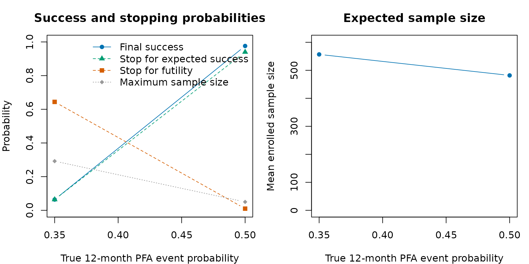
margin: PFA failure 50%	500	0	0.068	0.066	0.664	0.27	556.8
target: equal 35% failure	500	0	0.984	0.946	0.004	0.05	466.2

The table displays selected operating characteristics; oc_small retains the full summary, including Monte Carlo uncertainty. Each scenario uses 500 simulated trials and two cores. These results are illustrative rather than definitive estimates of power or type I error. A design evaluation should increase N_trials and N_impute as needed for Monte Carlo precision and examine sensitivity to accrual, loss to follow-up, event rates, and the imputation hazard model.

Graphical assessment of the simulated design

The plots answer complementary design questions. First, plot_sim_ocs() compares operating characteristics across the target and noninferiority-margin scenarios. The true PFA event probability is supplied as the effect scale.

effect_by_scenario <- c(
  "target: equal 35% failure" = 0.35,
  "margin: PFA failure 50%" = 0.50
)
oc_small$true_pfa_event_probability <- unname(
  effect_by_scenario[oc_small$scenario]
)
plot_sim_ocs(
  oc_small,
  effect = "true_pfa_event_probability",
  xlab = "True 12-month PFA event probability"
)

Within the target scenario, plot_sim_stopping() shows how often each sample size is selected and why enrollment stops.

plot_sim_stopping(eff_target)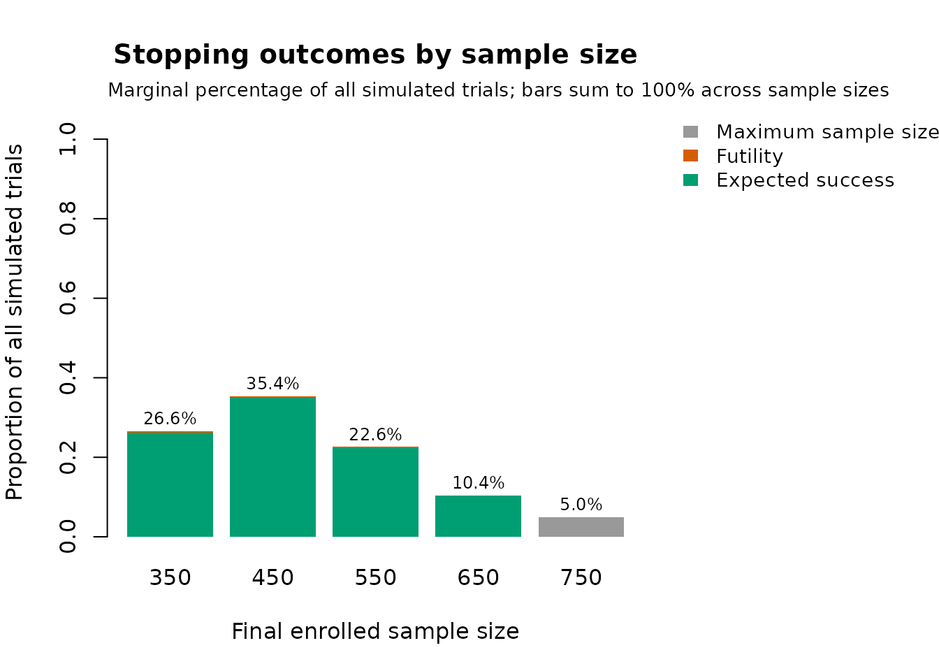

Because eff_target was simulated with return_trace = TRUE, its interim decision geometry can also be inspected. Each displayed panel corresponds to an ADVENT enrollment milestone reached in at least one simulated trial; larger bubbles represent predictive-probability pairs reached by more simulated trials.

plot_sim_decisions(eff_target)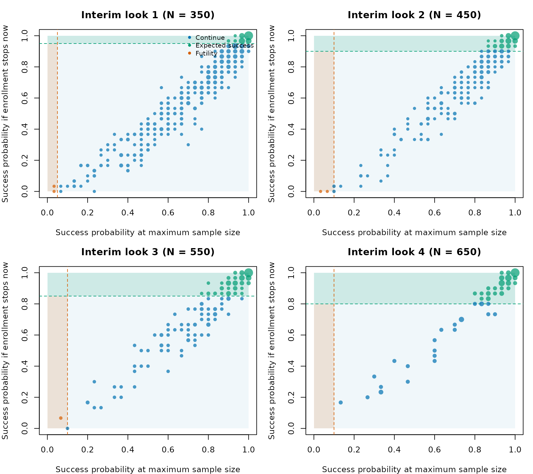

A fuller simulation template

The following larger simulation uses the ADVENT values of N_trials and N_impute. It is provided as a template and is not evaluated here.

advent_effectiveness_full_args <- modifyList(advent_effectiveness_args, list(
  N_impute = 5000,
  ncores = 8
))

advent_safety_full_args <- modifyList(advent_safety_args, list(
  N_impute = 5000,
  ncores = 8
))

eff_target_full <- do.call(sim_trials, c(
  advent_effectiveness_full_args,
  list(
    N_trials = 1000,
    hazard_treatment = eff_hazard_per_day,
    hazard_control = eff_hazard_per_day,
    h0 = 0.15,
    prob_ha = 0.956,
    seed = 4620
  )
))

eff_margin_full <- do.call(sim_trials, c(
  advent_effectiveness_full_args,
  list(
    N_trials = 1000,
    hazard_treatment = eff_margin_hazard_per_day,
    hazard_control = eff_hazard_per_day,
    h0 = 0.15,
    prob_ha = 0.956,
    seed = 4621
  )
))

safety_target_full <- do.call(sim_trials, c(
  advent_safety_full_args,
  list(
    N_trials = 1000,
    hazard_treatment = safety_hazard_per_day,
    hazard_control = safety_hazard_per_day,
    h0 = 0.08,
    prob_ha = 0.966,
    seed = 4622
  )
))

safety_margin_full <- do.call(sim_trials, c(
  advent_safety_full_args,
  list(
    N_trials = 1000,
    hazard_treatment = safety_margin_hazard_per_day,
    hazard_control = safety_hazard_per_day,
    h0 = 0.08,
    prob_ha = 0.966,
    seed = 4623
  )
))

summarise_sims(list(
  "effectiveness target" = eff_target_full,
  "effectiveness margin" = eff_margin_full,
  "safety target" = safety_target_full,
  "safety margin" = safety_margin_full
))

The “margin” scenarios above set the treatment event probability equal to the control event probability plus the noninferiority margin. They are useful for checking false-positive behavior near the design boundary. They are not the only null scenarios worth studying.

SAP sensitivity assumptions and reference benchmarks

The SAP assessed whether operating characteristics were robust to several alternative assumptions. In goldilocks notation, these correspond to:

Varying the day-360 event probability implied by the effectiveness hazard_control vector over c(0.40, 0.35, 0.30). These are failure probabilities and therefore correspond to the SAP’s control success probabilities of 0.60, 0.65, and 0.70. The day-360 event probability implied by the safety hazard_control vector was varied over c(0.06, 0.08, 0.10).
Supplying a slower lambda schedule of c(2, 5, 10, 10, 15, 15, 20, 25) / 30, with lambda_time = (1:7) * 30, or a faster schedule of c(5, 10, 20, 25, 30, 40, 50) / 30, with lambda_time = (1:6) * 30. Division by 30 converts the SAP’s subjects/month rates to the subjects/day scale used here.
Using the SAP’s second effectiveness generator with generation_cutpoints = c(90, 100, 200, 300) and both hazard_treatment and hazard_control set to c(0.000055695, 0.010034797, 0.001690763, 0.000680535, 0.000573122) in its equal-arm target scenario.
Using the SAP’s third effectiveness generator with generation_cutpoints = c(90, 120) and both hazard arguments set to c(0.000569925, 0.007879626, 0.000596254) in its equal-arm target scenario.
Using the SAP’s second safety generator with generation_cutpoints = c(7, 180) and both hazard arguments set to c(0.007327613, 0.000122991, 0.0000600610) in its equal-arm target scenario.

The three alternative event-time models deliberately use data-generating partitions that differ from the principal analysis partitions. They can be represented by changing generation_cutpoints and the hazard vectors while retaining cutpoints and the priors for the principal predictive model. The SAP also planned an imputation-model sensitivity with six pieces: day 90 followed by five post-90-day intervals containing approximately equal event counts, potentially with different cut-points by arm. goldilocks uses one analysis partition shared by both arms, so this arm-specific predictive model cannot currently be represented.

The SAP supplies quantitative reference results based on 10,000 simulated trials per scenario and M=5000 predictive draws or imputations:

Scenario	Reported probability	Probability meaning	Mean mITT sample size
Target: both endpoints at expected rates	0.9635	Joint power	504
Effectiveness noninferiority boundary	0.0487	Effectiveness type I error	551
Safety noninferiority boundary	0.0528	Safety type I error	457

The target row sets the effectiveness hazard_treatment and hazard_control vectors to imply equal day-360 failure probabilities of 0.35, and the safety hazard vectors to imply equal day-360 event probabilities of 0.08; success requires both co-primary endpoints. At the effectiveness boundary, hazard_treatment implies a 0.50 failure probability while hazard_control implies 0.35, and the safety endpoint was assumed always to recommend stopping for promise and to pass finally. At the safety boundary, the treatment and control safety hazards imply event probabilities of 0.16 and 0.08, respectively, and effectiveness was treated analogously. These are external validation targets. The endpoint-separated simulations in this vignette do not claim to reproduce them.

References

Broglio KR, Connor JT, Berry SM. Not too big, not too small: a Goldilocks approach to sample size selection. Journal of Biopharmaceutical Statistics. 2014;24(3):685-705. doi:10.1080/10543406.2014.888569.

Reddy VY, Gerstenfeld EP, Natale A, et al. A randomized controlled trial of pulsed field ablation versus standard-of-care ablation for paroxysmal atrial fibrillation: The ADVENT trial rationale and design. Heart Rhythm O2. 2023;4(5):317-328. doi:10.1016/j.hroo.2023.03.001.

Reddy VY, Gerstenfeld EP, Natale A, et al. Pulsed field or conventional thermal ablation for paroxysmal atrial fibrillation. New England Journal of Medicine. 2023;389(18):1660-1671. doi:10.1056/NEJMoa2307291.

ClinicalTrials.gov. A prospective randomized pivotal trial of the FARAPULSE pulsed field ablation system compared with standard of care ablation in patients with paroxysmal atrial fibrillation. NCT04612244.

FARAPULSE, Inc. ADVENT Statistical Analysis Plan. CS0935 Rev C. 12 October 2021. Available from the ClinicalTrials.gov document archive.