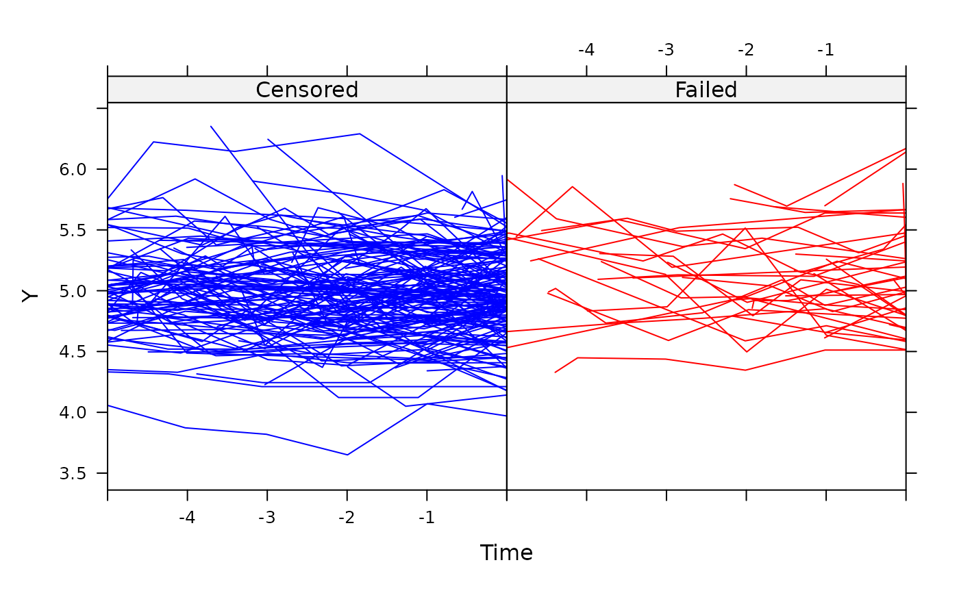
Joint plot of longitudinal and survival data

This function views the longitudinal profile of each unit with the last longitudinal measurement prior to event-time (censored or not) taken as the end-point, referred to as time zero. In doing so, the shape of the profile prior to event-time can be inspected. This can be done over a user-specified number of time units.

Usage

jointplot(
  object,
  Y.col,
  Cens.col,
  lag,
  split = TRUE,
  col1,
  col2,
  xlab,
  ylab,
  gp1lab,
  gp2lab,
  smooth = 2/3,
  mean.profile = FALSE,
  mcol1,
  mcol2
)

Arguments

object: an object of class jointdata.
Y.col: an element of class character identifying the longitudinal response part of the jointdata object.
Cens.col: an element of class character identifying the survival status or censoring indicator part of the jointdata object.
lag: argument which specifies how many units in time we look back through. Defaults to the maximum observation time across all units.
split: logical argument which allows the profiles of units which fail and those which are censored to be viewed in separate panels of the same graph. This is the default option. Using split = FALSE will plot all profiles overlaid on a single plot.
col1: argument to choose the colour for the profiles of the censored units.
col2: argument to choose the colour for the profiles of the failed units.
xlab: an element of class character indicating the title for the x-axis.
ylab: an element of class character indicating the title for the y-axis.
gp1lab: an element of class character for the group corresponding to a censoring indicator of zero. Typically, the censored group.
gp2lab: an element of class character for the group corresponding to a censoring indicator of one. Typically, the group experiencing the event of interest.
smooth: the smoother span. This gives the proportion of points in the plot which influence the smooth at each value. Defaults to a value of 2/3. Larger values give more smoothness. See lowess for further details.
mean.profile: draw mean profiles if TRUE. Only applies to the split = TRUE case.
mcol1: argument to choose the colour for the mean profile of the units with a censoring indicator of zero.
mcol2: argument to choose the colour for the mean profile of the units with a censoring indicator of one.

Value

A lattice plot.

Details

The function tailors the xyplot function to produce a representation of joint data with longitudinal and survival components.

Note

If more than one cause of failure is present (i.e. competing risks data), then all failures are pooled together into a single failure type.

References

Wulfsohn MS, Tsiatis AA. A joint model for survival and longitudinal data measured with error. Biometrics. 1997; 53(1): 330-339.

Author

Pete Philipson

Examples

data(heart.valve)
heart.surv <- UniqueVariables(heart.valve,
                              var.col = c("fuyrs", "status"),
                              id.col = "num")
heart.long <- heart.valve[, c("num", "time", "log.lvmi")]
heart.cov <- UniqueVariables(heart.valve,
                             c("age", "sex"),
                             id.col = "num")
heart.valve.jd <- jointdata(longitudinal = heart.long,
                            baseline = heart.cov,
                            survival = heart.surv,
                            id.col = "num",
                            time.col = "time")
jointplot(heart.valve.jd, Y.col = "log.lvmi",
          Cens.col = "status", lag = 5)