Calibrating `prob_ha` for type I error control • goldilocks

library(goldilocks)

The decision thresholds in a Goldilocks design are not guarantees of its frequentist operating characteristics. In particular, setting prob_ha = 0.975 does not by itself guarantee that the complete adaptive design has one-sided type I error no greater than 0.025. Interim analyses, predictive stopping, the enrollment and follow-up processes, and the Monte Carlo settings all contribute to the probability of a successful trial under the null hypothesis.

This vignette demonstrates a focused calibration procedure:

Prespecify a null data-generating scenario and a target type I error.
Screen a finite grid of prob_ha values while holding the rest of the design fixed.
Use Monte Carlo intervals to distinguish controlled, uncontrolled, and inconclusive candidates.
Validate the selected candidate with more simulations and a fresh seed.

The result is evidence about the simulated scenarios, not a mathematical guarantee over every possible data-generating process. A design with a composite null may require several prespecified nuisance-parameter scenarios.

Design and null scenario

The example uses a two-arm design with a one-sided log-rank analysis. Both arms have a 30% event probability by 12 months under the null. The design permits futility stopping and stopping accrual for expected success, but does not permit an immediate success claim at an interim look because Qn = 1.

target_type1 <- 0.025
prob_ha_grid <- seq(0.965, 0.995, by = 0.005)
null_hazard <- prop_to_haz(0.30, endtime = 12)

calibration_design <- list(
  hazard_treatment = null_hazard,
  hazard_control = null_hazard,
  cutpoints = NULL,
  N_total = 300,
  lambda = 5,
  lambda_time = NULL,
  interim_look = seq(100, 275, 25),
  end_of_study = 12,
  prior_surv = c(0.1, 0.1),
  block = 2,
  rand_ratio = c(control = 1, treatment = 1),
  prop_loss = 0,
  alternative = "less",
  h0 = 0,
  Fn = rep(0.10, 8),
  Sn = c(1, rep(0.90, 7)),
  Qn = 1,
  N_impute = 100,
  method = "logrank",
  return_trace = FALSE,
  ncores = 8
)

Only prob_ha changes across candidates. In particular, N_impute is fixed: it is part of the implemented interim decision algorithm, not merely a precision setting for this calibration exercise. The number of simulated trials, N_trials, controls the Monte Carlo precision of the estimated operating characteristics and can be increased during validation.

Screening a candidate grid

The following code runs 2,000 null trials for every candidate. These calculations are performed offline for the built vignette; their compact summaries are loaded from the accompanying data file.

screening_seed <- 67201

screening_results <- lapply(prob_ha_grid, function(threshold) {
  do.call(
    sim_trials,
    c(
      calibration_design,
      list(
        prob_ha = threshold,
        N_trials = 2000,
        seed = screening_seed
      )
    )
  )
})
names(screening_results) <- sprintf("prob_ha = %.3f", prob_ha_grid)

screening_summary <- summarise_sims(screening_results)
screening_summary$prob_ha <- prob_ha_grid

The same seed is deliberately used for each candidate. Because the candidates differ only in prob_ha, this applies common random numbers and reduces irrelevant Monte Carlo variation in the screening curve. Candidate results are therefore correlated, and their marginal Monte Carlo intervals should not be interpreted as confidence intervals for pairwise differences.

Under the null, the power column returned by summarise_sims() is the estimated type I error. Its power_mc_lower and power_mc_upper columns form a 95% Wilson Monte Carlo interval. We apply the following deliberately conservative screening rule:

controlled: the upper Monte Carlo bound is at or below the target;
not controlled: the lower bound is above the target; and
inconclusive: the interval overlaps the target.

classify_type1 <- function(summary, target) {
  ifelse(
    summary$power_mc_upper <= target,
    "controlled",
    ifelse(
      summary$power_mc_lower > target,
      "not controlled",
      "inconclusive"
    )
  )
}

calibration_screening$type1_status <- classify_type1(
  calibration_screening,
  target_type1
)

screening_display <- calibration_screening[c(
  "prob_ha",
  "n_used",
  "power",
  "power_mc_lower",
  "power_mc_upper",
  "type1_status"
)]
names(screening_display)[3:5] <- c(
  "type1_error",
  "type1_mc_lower",
  "type1_mc_upper"
)
knitr::kable(screening_display, digits = 3)

prob_ha	n_used	type1_error	type1_mc_lower	type1_mc_upper	type1_status
0.965	2000	0.044	0.036	0.054	not controlled
0.970	2000	0.035	0.028	0.045	not controlled
0.975	2000	0.032	0.025	0.041	not controlled
0.980	2000	0.024	0.018	0.031	inconclusive
0.985	2000	0.018	0.013	0.024	controlled
0.990	2000	0.012	0.008	0.017	controlled
0.995	2000	0.006	0.004	0.011	controlled

Plotting the calibration curve

The shaded area is at or below the target type I error. A candidate is classified as controlled only when its entire displayed Monte Carlo interval falls in that region.

screening_plot <- calibration_screening[
  order(calibration_screening$prob_ha),
]
status_colours <- c(
  "controlled" = "#009E73",
  "inconclusive" = "#E69F00",
  "not controlled" = "#D55E00"
)
point_colours <- unname(status_colours[screening_plot$type1_status])
y_max <- max(screening_plot$power_mc_upper, target_type1) * 1.08

plot(
  screening_plot$prob_ha,
  screening_plot$power,
  type = "n",
  ylim = c(0, y_max),
  xlab = expression(prob[ha]),
  ylab = "Null rejection probability (estimated type I error)",
  main = "Screening prob_ha against a 0.025 target"
)
plot_region <- par("usr")
rect(
  plot_region[1],
  0,
  plot_region[2],
  target_type1,
  col = grDevices::adjustcolor("#009E73", alpha.f = 0.10),
  border = NA
)
abline(h = target_type1, col = "#0072B2", lty = 2, lwd = 2)
lines(screening_plot$prob_ha, screening_plot$power, col = "#555555")
arrows(
  screening_plot$prob_ha,
  screening_plot$power_mc_lower,
  screening_plot$prob_ha,
  screening_plot$power_mc_upper,
  angle = 90,
  code = 3,
  length = 0.04,
  col = point_colours
)
points(
  screening_plot$prob_ha,
  screening_plot$power,
  pch = 19,
  col = point_colours
)
legend(
  "topright",
  legend = c(names(status_colours), "target"),
  col = c(unname(status_colours), "#0072B2"),
  pch = c(19, 19, 19, NA),
  lty = c(NA, NA, NA, 2),
  bty = "n"
)

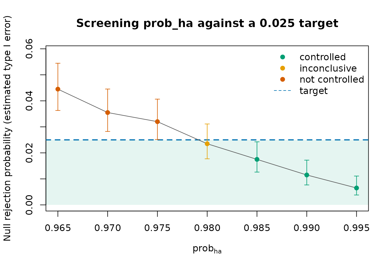
Estimated type I error and 95% Monte Carlo intervals across seven prob_ha candidates. The intervals for candidates 0.985, 0.990, and 0.995 fall below the horizontal 0.025 target.

The grid is discrete, so this plot does not justify interpolation to an untested value. Nor is the curve required to be perfectly monotone: changing prob_ha changes completed-data success classifications, predictive stopping, and potentially the final sample size. Here we select the smallest screened value classified as controlled, rather than claiming it is the unique or optimal threshold.

controlled_candidates <- calibration_screening$prob_ha[
  calibration_screening$type1_status == "controlled"
]
if (length(controlled_candidates) == 0L) {
  stop("No screened candidate meets the Monte Carlo criterion; revise the grid or simulation size.")
}
selected_prob_ha <- min(controlled_candidates)
selected_prob_ha
#> [1] 0.985

Independent validation

Selecting a candidate because it performed well in the screening simulations introduces selection bias. The selected design should therefore be rerun with a fresh simulation seed. The validation below keeps all prespecified decision settings fixed and increases only N_trials, from 2,000 to 10,000.

validation_result <- do.call(
  sim_trials,
  c(
    calibration_design,
    list(
      prob_ha = selected_prob_ha,
      N_trials = 10000,
      seed = 67202
    )
  )
)

validation_summary <- summarise_sims(list(
  "fresh-seed validation" = validation_result
))
validation_summary$prob_ha <- selected_prob_ha
validation_summary$type1_status <- classify_type1(
  validation_summary,
  target_type1
)

validation_display <- calibration_validation[c(
  "prob_ha",
  "n_used",
  "power",
  "power_mc_lower",
  "power_mc_upper",
  "type1_status"
)]
names(validation_display)[3:5] <- c(
  "type1_error",
  "type1_mc_lower",
  "type1_mc_upper"
)
knitr::kable(validation_display, digits = 4)

prob_ha	n_used	type1_error	type1_mc_lower	type1_mc_upper	type1_status
0.985	10000	0.0182	0.0158	0.021	controlled

The fresh-seed validation is the relevant assessment of the selected candidate. If it is inconclusive or not controlled, the candidate set or simulation size should be reconsidered and another independent validation planned; repeatedly selecting against the same validation simulations would turn them into an extension of the screening data.

Extending the calibration

For a target of 0.05, change target_type1 and choose a grid appropriate to that target. Do not assume that prob_ha = 1 - target_type1 controls the type I error of the full adaptive design.

When the null contains nuisance parameters, repeat the candidate grid for each prespecified null scenario. A simple conservative requirement is that the upper Monte Carlo bound be below the target in every scenario. This establishes simulation evidence only on that finite scenario set; identifying a least-favourable configuration and accounting for searches over many scenarios remain design-specific statistical responsibilities.

After calibrating type I error, simulate the selected design under one or more clinically relevant alternative scenarios to estimate power and expected sample size. Those simulations should retain the selected prob_ha and the same prespecified values of N_impute and N_mcmc intended for the trial.

Calibrating an RMST design

The workflow also applies to method = "rmst", but the null is defined on the treatment-minus-control RMST scale. The following specification keeps the equal-hazard null from the example and targets a difference of zero through month nine, with follow-up continuing through month twelve:

rmst_calibration_design <- modifyList(calibration_design, list(
  method = "rmst",
  rmst_tau = 9,
  alternative = "greater",
  h0 = 0
))

Repeat screening and independent validation with this design in place of calibration_design; the stored log-rank results and selected threshold do not calibrate RMST. Keep rmst_tau fixed throughout the search. When allowing a loss of m months for non-inferiority, use h0 = -m and generate boundary-null scenarios with a true RMST difference of -m at that horizon.

Equal survival distributions provide one zero-difference null scenario. Crossing survival curves can also have equal RMST, so evaluate those scenarios when relevant, together with dropout and discrepancies between generation_cutpoints and the predictive cutpoints. Inspect failure counts as well as rejection rates: inadequate support through the fixed horizon or zero total variance can make an RMST analysis non-estimable. The RMST vignette describes these requirements and gives executable trial simulations.